drivingScenario
Create driving scenario
Description
The drivingScenario object represents a 3-D
arena containing roads, parking lots, vehicles, pedestrians, barriers, and other aspects
of a driving scenario. Use this object to model realistic traffic scenarios and to
generate synthetic detections for testing controllers or sensor fusion
algorithms.
To add roads, use the
roadfunction. To specify lanes in the roads, create alanespecobject. You can also import roads from a third-party road network by using theroadNetworkfunction.To add parking lots, use the
parkingLotfunction.To add actors (cars, pedestrians, bicycles, and so on), use the
actorfunction. To add actors with properties designed specifically for vehicles, use thevehiclefunction. To add barriers, use thebarrierfunction. All actors, including vehicles and barriers, are modeled as cuboids (box shapes) with unique actor IDs.To simulate a scenario, call the
advancefunction in a loop, which advances the simulation one time step at a time.
You can also create driving scenarios interactively by using the Driving Scenario
Designer app. In addition, you can export drivingScenario
objects from the app to produce scenario variations for use in either the app or in
Simulink®.
Creation
Description
scenario = drivingScenario
scenario = drivingScenario(Name,Value)SampleTime, StopTime,
and GeoReference properties using name-value pairs. For
example, drivingScenario('GeoReference',[42.3 -71.0 0]) sets
the geographic origin of the scene to a latitude-longitude coordinate of (42.3,
–71.0) and an altitude of 0.
Properties
Object Functions
Examples
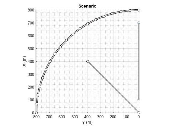
Create a driving scenario containing a curved road, two straight roads, and two actors: a car and a bicycle. Both actors move along the road for 60 seconds.
Create the driving scenario object.
scenario = drivingScenario('SampleTime',0.1','StopTime',60);
Create the curved road using road center points following the arc of a circle with an 800-meter radius. The arc starts at 0°, ends at 90°, and is sampled at 5° increments.
angs = [0:5:90]';
R = 800;
roadcenters = R*[cosd(angs) sind(angs) zeros(size(angs))];
roadwidth = 10;
cr = road(scenario,roadcenters,roadwidth);
Add two straight roads with the default width, using road center points at each end. To the first straight road add barriers on both road edges.
roadcenters = [700 0 0; 100 0 0];
sr1 = road(scenario,roadcenters);
barrier(scenario,sr1)
barrier(scenario,sr1,'RoadEdge','left')
roadcenters = [400 400 0; 0 0 0];
road(scenario,roadcenters);
Get the road boundaries.
rbdry = roadBoundaries(scenario);
Add a car and a bicycle to the scenario. Position the car at the beginning of the first straight road.
car = vehicle(scenario,'ClassID',1,'Position',[700 0 0], ...
    'Length',3,'Width',2,'Height',1.6);
Position the bicycle farther down the road.
bicycle = actor(scenario,'ClassID',3,'Position',[706 376 0]', ...
    'Length',2,'Width',0.45,'Height',1.5);
Plot the scenario.
plot(scenario,'Centerline','on','RoadCenters','on');
title('Scenario');
Display the actor poses and profiles.
allActorPoses = actorPoses(scenario)
allActorPoses=242×1 struct array with fields:
    ActorID
    Position
    Velocity
    Roll
    Pitch
    Yaw
    AngularVelocity
allActorProfiles = actorProfiles(scenario)
allActorProfiles=242×1 struct array with fields:
    ActorID
    ClassID
    Length
    Width
    Height
    OriginOffset
    MeshVertices
    MeshFaces
    RCSPattern
    RCSAzimuthAngles
    RCSElevationAngles
Because there are barriers in this scenario, and each barrier segment is considered an actor, actorPoses and actorProfiles functions return the poses of all stationary and non-stationary actors. To only obtain the poses and profiles of non-stationary actors such as vehicles and bicycles, first obtain their corresponding actor IDs using the scenario.Actors.ActorID property.
movableActorIDs = [scenario.Actors.ActorID];
Then, use those IDs to filter only non-stationary actor poses and profiles.
movableActorPoseIndices = ismember([allActorPoses.ActorID],movableActorIDs);

movableActorPoses = allActorPoses(movableActorPoseIndices)
movableActorPoses=2×1 struct array with fields:
    ActorID
    Position
    Velocity
    Roll
    Pitch
    Yaw
    AngularVelocity
movableActorProfiles = allActorProfiles(movableActorPoseIndices)
movableActorProfiles=2×1 struct array with fields:
    ActorID
    ClassID
    Length
    Width
    Height
    OriginOffset
    MeshVertices
    MeshFaces
    RCSPattern
    RCSAzimuthAngles
    RCSElevationAngles
Create a driving scenario and show how target outlines change as the simulation advances.
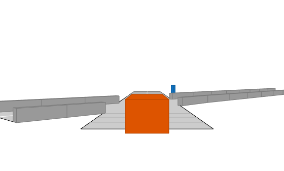
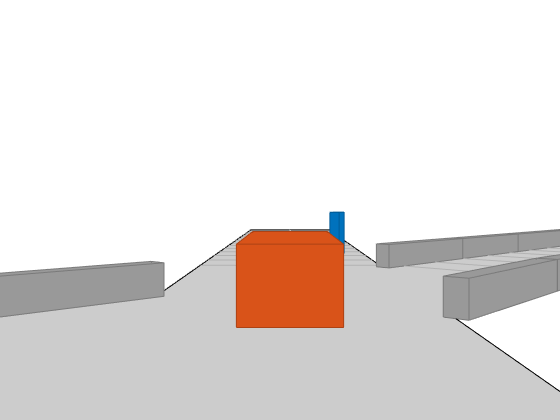
Create a driving scenario consisting of two intersecting straight roads. The first road segment is 45 meters long. The second straight road is 32 meters long with jersey barriers along both its edges, and intersects the first road. A car traveling at 12.0 meters per second along the first road approaches a running pedestrian crossing the intersection at 2.0 meters per second.
scenario = drivingScenario('SampleTime',0.1,'StopTime',1);
road1 = road(scenario,[-10 0 0; 45 -20 0]);
road2 = road(scenario,[-10 -10 0; 35 10 0]);
barrier(scenario,road1)
barrier(scenario,road1,'RoadEdge','left')
ped = actor(scenario,'ClassID',4,'Length',0.4,'Width',0.6,'Height',1.7);
car = vehicle(scenario,'ClassID',1);
pedspeed = 2.0;
carspeed = 12.0;
smoothTrajectory(ped,[15 -3 0; 15 3 0],pedspeed);
smoothTrajectory(car,[-10 -10 0; 35 10 0],carspeed);
Create an ego-centric chase plot for the vehicle.
chasePlot(car,'Centerline','on')
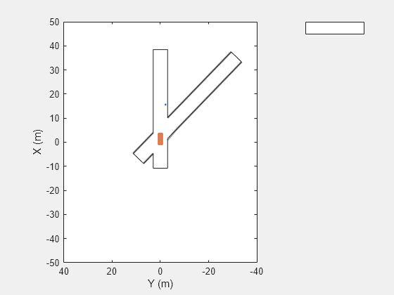
Create an empty bird's-eye plot and add an outline plotter and lane boundary plotter. Then, run the simulation. At each simulation step:
Update the chase plot to display the road boundaries and target outlines.
Update the bird's-eye plot to display the updated road boundaries and target outlines. The plot perspective is always with respect to the ego vehicle.
bepPlot = birdsEyePlot('XLim',[-50 50],'YLim',[-40 40]);
outlineplotter = outlinePlotter(bepPlot);
laneplotter = laneBoundaryPlotter(bepPlot);
legend('off')

while advance(scenario)
    rb = roadBoundaries(car);
    [position,yaw,length,width,originOffset,color] = targetOutlines(car);
    [bposition,byaw,blength,bwidth,boriginOffset,bcolor,barrierSegments] = targetOutlines(car,'Barriers');
    plotLaneBoundary(laneplotter,rb)
    plotOutline(outlineplotter,position,yaw,length,width, ...
        'OriginOffset',originOffset,'Color',color)
    plotBarrierOutline(outlineplotter,barrierSegments,bposition,byaw,blength,bwidth, ...
        'OriginOffset',boriginOffset,'Color',bcolor)
    pause(0.01)
end
Create a driving scenario containing an ego vehicle and a target vehicle traveling along a three-lane road. Detect the lane boundaries by using a vision detection generator.
scenario = drivingScenario;
Create a three-lane road by using lane specifications.
roadCenters = [0 0 0; 60 0 0; 120 30 0];
lspc = lanespec(3);
road(scenario,roadCenters,'Lanes',lspc);
Specify that the ego vehicle follows the center lane at 30 m/s.
egovehicle = vehicle(scenario,'ClassID',1);
egopath = [1.5 0 0; 60 0 0; 111 25 0];
egospeed = 30;
smoothTrajectory(egovehicle,egopath,egospeed);
Specify that the target vehicle travels ahead of the ego vehicle at 40 m/s and changes lanes close to the ego vehicle.
targetcar = vehicle(scenario,'ClassID',1);
targetpath = [8 2; 60 -3.2; 120 33];
targetspeed = 40;
smoothTrajectory(targetcar,targetpath,targetspeed);
Display a chase plot for a 3-D view of the scenario from behind the ego vehicle.
chasePlot(egovehicle)

Create a vision detection generator that detects lanes and objects. The pitch of the sensor points one degree downward.
visionSensor = visionDetectionGenerator('Pitch',1.0);
visionSensor.DetectorOutput = 'Lanes and objects';
visionSensor.ActorProfiles = actorProfiles(scenario);
Run the simulation.
Create a bird's-eye plot and the associated plotters.
Display the sensor coverage area.
Display the lane markings.
Obtain ground truth poses of targets on the road.
Obtain ideal lane boundary points up to 60 m ahead.
Generate detections from the ideal target poses and lane boundaries.
Display the outline of the target.
Display object detections when the object detection is valid.
Display the lane boundary when the lane detection is valid.
bep = birdsEyePlot('XLim',[0 60],'YLim',[-35 35]);
caPlotter = coverageAreaPlotter(bep,'DisplayName','Coverage area', ...
    'FaceColor','blue');
detPlotter = detectionPlotter(bep,'DisplayName','Object detections');
lmPlotter = laneMarkingPlotter(bep,'DisplayName','Lane markings');
lbPlotter = laneBoundaryPlotter(bep,'DisplayName', ...
    'Lane boundary detections','Color','red');
olPlotter = outlinePlotter(bep);
plotCoverageArea(caPlotter,visionSensor.SensorLocation,...
    visionSensor.MaxRange,visionSensor.Yaw, ...
    visionSensor.FieldOfView(1));
while advance(scenario)
    [lmv,lmf] = laneMarkingVertices(egovehicle);
    plotLaneMarking(lmPlotter,lmv,lmf)
    tgtpose = targetPoses(egovehicle);
    lookaheadDistance = 0:0.5:60;
    lb = laneBoundaries(egovehicle,'XDistance',lookaheadDistance,'LocationType','inner');
    [obdets,nobdets,obValid,lb_dets,nlb_dets,lbValid] = ...
        visionSensor(tgtpose,lb,scenario.SimulationTime);
    [objposition,objyaw,objlength,objwidth,objoriginOffset,color] = targetOutlines(egovehicle);
    plotOutline(olPlotter,objposition,objyaw,objlength,objwidth, ...
        'OriginOffset',objoriginOffset,'Color',color)
    if obValid
        detPos = cellfun(@(d)d.Measurement(1:2),obdets,'UniformOutput',false);
        detPos = vertcat(zeros(0,2),cell2mat(detPos')');
        plotDetection(detPlotter,detPos)
    end
    if lbValid
        plotLaneBoundary(lbPlotter,vertcat(lb_dets.LaneBoundaries))
    end
end


In this example, you will add sensors to a driving scenario using the addSensors function and get ground-truth target poses based on the individual sensor inputs. Then, you process the ground-truth target poses into detections and visualize them.
Set Up Driving Scenario and Bird's-Eye-Plot
Create a driving scenario with an ego vehicle and two target vehicles. One target vehicle is in the front and the other is to the left of the ego-vehicle.
[scenario, egovehicle] = helperCreateDrivingScenario;
Configure a vision sensor to be mounted at the front of the ego vehicle.
visionSensor = visionDetectionGenerator(SensorIndex=1,SensorLocation=[4.0 0],Height=1.1,Pitch=1.0,DetectorOutput="Objects only");Configure an ultrasonic sensor to be mounted at the left side of the ego-vehicle.
leftUltrasonic = ultrasonicDetectionGenerator(SensorIndex=2,MountingLocation=[0.5 1 0.2],MountingAngles=[90 0 0],FieldOfView=[70 35],UpdateRate=100);
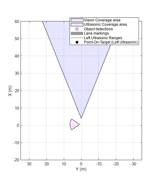
Create a bird's-eye-plot to visualize the driving scenario.
figHandle=figure(Name="BEP",Visible="on");
[detPlotter,lmPlotter,olPlotter,lulrdPlotter,luldetPlotter] = helperCreateBEP(visionSensor,leftUltrasonic,figHandle);
Add Sensors and Simulate Driving Scenario
Add both vision and ultrasonic sensors to the driving scenario using the addSensors function. You can add sensors to any vehicle in the driving scenario using the addSensors function by specifying the actor ID of the desired vehicle. In this example, specify the ego-vehicle actor ID.
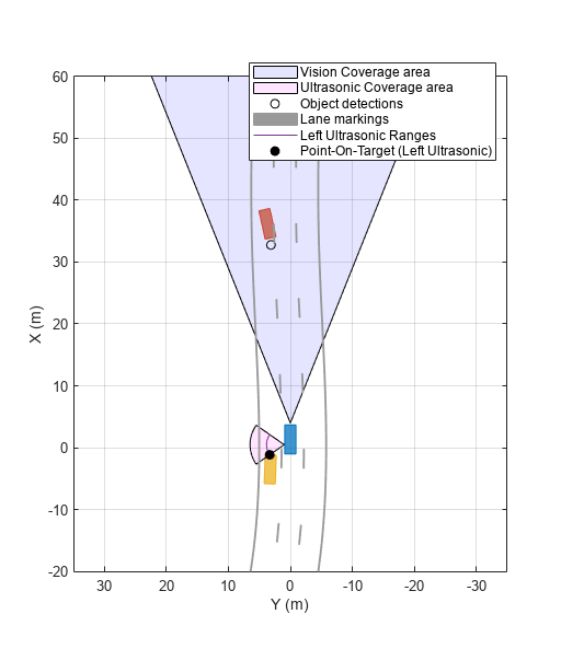
addSensors(scenario,{visionSensor,leftUltrasonic},egovehicle.ActorID);Simulate the driving scenario. Note that you get separate target poses based on individual sensors by specifying their respective sensor IDs as inputs to the targetPoses function. This syntax returns the ground-truth poses of targets only within the range of the specified sensor. You then pass the ground-truth poses to their respective sensor models to generate detections and visualize them.
while advance(scenario)
    % Plot scenario lane markings and vehicle outlines at current timestep
    [lmv,lmf] = laneMarkingVertices(egovehicle);
    plotLaneMarking(lmPlotter,lmv,lmf)
    [objposition,objyaw,objlength,objwidth,objoriginOffset,color] = targetOutlines(egovehicle);
    plotOutline(olPlotter,objposition,objyaw,objlength,objwidth, ...
        OriginOffset=objoriginOffset,Color=color)

    % Get ground-truth poses of targets in the range of vision and ultrasonic sensors separately
    tgtposeVision = targetPoses(scenario,visionSensor.SensorIndex);
    tgtposeUltrasonic = targetPoses(scenario,leftUltrasonic.SensorIndex);

    % Obtain detections based on targets only in range
    [obdets,obValid] = visionSensor(tgtposeVision,scenario.SimulationTime);
    [lobdets,lobValid] = leftUltrasonic(tgtposeUltrasonic,scenario.SimulationTime);

    helperPlotBEPVision(obdets,obValid,detPlotter)
    helperPlotBEPUltrasonic(lobdets,lobValid,leftUltrasonic,lulrdPlotter,luldetPlotter)
end
Helper Functions
helperCreateDrivingScenario creates a driving scenario by specifying the road and vehicle properties.
function [scenario, egovehicle] = helperCreateDrivingScenario
    scenario = drivingScenario;
    roadCenters = [-120 30 0;-60 0 0;0 0 0; 60 0 0; 120 30 0; 180 60 0];
    lspc = lanespec(3);
    road(scenario,roadCenters,Lanes=lspc);

    % Create an ego vehicle that travels in the center lane at a velocity of 30 m/s.
    egovehicle = vehicle(scenario,ClassID=1);
    egopath = [1.5 0 0; 60 0 0; 111 25 0];
    egospeed = 30;
    smoothTrajectory(egovehicle,egopath,egospeed);

    % Add a target vehicle that travels ahead of the ego vehicle at 30.5 m/s in the right lane, and changes lanes close to the ego vehicle.
    ftargetcar = vehicle(scenario,ClassID=1);
    ftargetpath = [8 2; 60 -3.2; 120 33];
    ftargetspeed = 40;
    smoothTrajectory(ftargetcar,ftargetpath,ftargetspeed);

    % Add a second target vehicle that travels in the left lane at 32m/s.
    ltargetcar = vehicle(scenario,ClassID=1);
    ltargetpath = [-5.0 3.5 0; 60 3.5 0; 111 28.5 0];
    ltargetspeed = 30;
    smoothTrajectory(ltargetcar,ltargetpath,ltargetspeed);
end
helperCreateBEP creates a bird's-eye-plot for visualizing the driving scenario simulation.
function [detPlotter, lmPlotter, olPlotter, lulrdPlotter,luldetPlotter] = helperCreateBEP(visionSensor,leftUltrasonic,Figure)

    screenSize = double(get(groot,'ScreenSize'));
    Figure.Position = [screenSize(3)*0.17 screenSize(4)*0.15 screenSize(3)*0.4 screenSize(4)*0.6];
    clf(Figure);
    bepAxes = axes(Figure);
    grid(bepAxes,'on');

    bep = birdsEyePlot(Parent=bepAxes,XLim=[-20 60],YLim=[-35 35]);
    caPlotterV = coverageAreaPlotter(bep,DisplayName="Vision Coverage area",FaceColor="b");
    caPlotterU = coverageAreaPlotter(bep,DisplayName="Ultrasonic Coverage area",FaceColor="m");
    detPlotter = detectionPlotter(bep,DisplayName="Object detections");
    lmPlotter = laneMarkingPlotter(bep,DisplayName="Lane markings");
    olPlotter = outlinePlotter(bep);
    plotCoverageArea(caPlotterV,visionSensor.SensorLocation,...
        visionSensor.MaxRange,visionSensor.Yaw, ...
        visionSensor.FieldOfView(1));
    plotCoverageArea(caPlotterU,leftUltrasonic.MountingLocation(1:2),...
        leftUltrasonic.DetectionRange(3),leftUltrasonic.MountingAngles(1), ...
        leftUltrasonic.FieldOfView(1));

    lulrdPlotter = rangeDetectionPlotter(bep,DisplayName="Left Ultrasonic Ranges",LineStyle="-");
    luldetPlotter = detectionPlotter(bep,DisplayName="Point-On-Target (Left Ultrasonic)",MarkerFaceColor="k");
end
helperPlotBEPVision plots vision detections on the bird's-eye-plot.
function helperPlotBEPVision(obdets,obValid,detPlotter)

    if obValid
        detPos = cellfun(@(d)d.Measurement(1:2),obdets,UniformOutput=false);
        detPos = vertcat(zeros(0,2),cell2mat(detPos')');
        plotDetection(detPlotter,detPos)
    end

end
helperPlotBEPUltrasonic plots ultrasonic range measurements and points on targets.
function helperPlotBEPUltrasonic(lobdets,lobValid,leftUltrasonic,lulrdPlotter,luldetPlotter)

    if ~isempty(lobdets) && lobValid
        lranges = lobdets{1}.Measurement;
        plotRangeDetection(lulrdPlotter,lranges,leftUltrasonic.FieldOfView(1),leftUltrasonic.MountingLocation,leftUltrasonic.MountingAngles)
        plotDetection(luldetPlotter,lobdets{1}.ObjectAttributes{1}.PointOnTarget(1:2)')
    end

end