Main Content

insSensor

Inertial navigation system and GNSS/GPS simulation model

Since R2021a

Description

The insSensor System object™ models a device that fuses measurements from an inertial navigation system (INS) and global navigation satellite system (GNSS) such as a GPS, and outputs the fused measurements.

To output fused INS and GNSS measurements:

  1. Create the insSensor object and set its properties.

  2. Call the object with arguments, as if it were a function.

To learn more about how System objects work, see What Are System Objects?

Creation

Description

example

INS = insSensor returns a System object, INS, that models a device that outputs measurements from an INS and GNSS.

INS = insSensor(Name,Value) sets properties using one or more name-value pairs. Unspecified properties have default values. Enclose each property name in quotes.

Properties

expand all

Unless otherwise indicated, properties are nontunable, which means you cannot change their values after calling the object. Objects lock when you call them, and the release function unlocks them.

If a property is tunable, you can change its value at any time.

For more information on changing property values, see System Design in MATLAB Using System Objects.

Location of the sensor on the platform, in meters, specified as a three-element real-valued vector of the form [x y z]. The vector defines the offset of the sensor origin from the origin of the platform.

Tunable: Yes

Data Types: single | double

Accuracy of the roll measurement of the sensor body, in degrees, specified as a nonnegative real scalar.

Roll is the rotation around the x-axis of the sensor body. Roll noise is modeled as a white noise process. RollAccuracy sets the standard deviation of the roll measurement noise.

Tunable: Yes

Data Types: single | double

Accuracy of the pitch measurement of the sensor body, in degrees, specified as a nonnegative real scalar.

Pitch is the rotation around the y-axis of the sensor body. Pitch noise is modeled as a white noise process. PitchAccuracy defines the standard deviation of the pitch measurement noise.

Tunable: Yes

Data Types: single | double

Accuracy of the yaw measurement of the sensor body, in degrees, specified as a nonnegative real scalar.

Yaw is the rotation around the z-axis of the sensor body. Yaw noise is modeled as a white noise process. YawAccuracy defines the standard deviation of the yaw measurement noise.

Tunable: Yes

Data Types: single | double

Accuracy of the position measurement of the sensor body, in meters, specified as a nonnegative real scalar or a three-element real-valued vector. The elements of the vector set the accuracy of the x-, y-, and z-position measurements, respectively. If you specify PositionAccuracy as a scalar value, then the object sets the accuracy of all three positions to this value.

Position noise is modeled as a white noise process. PositionAccuracy defines the standard deviation of the position measurement noise.

Tunable: Yes

Data Types: single | double

Accuracy of the velocity measurement of the sensor body, in meters per second, specified as a nonnegative real scalar.

Velocity noise is modeled as a white noise process. VelocityAccuracy defines the standard deviation of the velocity measurement noise.

Tunable: Yes

Data Types: single | double

Accuracy of the acceleration measurement of the sensor body, in meters per second, specified as a nonnegative real scalar.

Acceleration noise is modeled as a white noise process. AccelerationAccuracy defines the standard deviation of the acceleration measurement noise.

Tunable: Yes

Data Types: single | double

Accuracy of the angular velocity measurement of the sensor body, in meters per second, specified as a nonnegative real scalar.

Angular velocity is modeled as a white noise process. AngularVelocityAccuracy defines the standard deviation of the acceleration measurement noise.

Tunable: Yes

Data Types: single | double

Enable input of simulation time, specified as a logical 0 (false) or 1 (true). Set this property to true to input the simulation time by using the simTime argument.

Tunable: No

Data Types: logical

Enable GNSS fix, specified as a logical 1 (true) or 0 (false). Set this property to false to simulate the loss of a GNSS receiver fix. When a GNSS receiver fix is lost, position measurements drift at a rate specified by the PositionErrorFactor property.

Tunable: Yes

Dependencies

To enable this property, set TimeInput to true.

Data Types: logical

Position error factor without GNSS fix, specified as a scalar or a 1-by-3 vector of scalars.

When the HasGNSSFix property is set to false, the position error grows at a quadratic rate due to constant bias in the accelerometer. The position error for a position component E(t) can be expressed as E(t) = 1/2αt2, where α is the position error factor for the corresponding component and t is the time since the GNSS fix is lost. While running, the object computes t based on the simTime input. The computed E(t) values for the x, y, and z components are added to the corresponding position components of the gTruth input.

Tunable: Yes

Dependencies

To enable this property, set TimeInput to true and HasGNSSFix to false.

Data Types: single | double

Random number source, specified as one of these options:

  • 'Global stream' –– Generate random numbers using the current global random number stream.

  • 'mt19937ar with seed' –– Generate random numbers using the mt19937ar algorithm, with the seed specified by the Seed property.

Data Types: char | string

Initial seed of the mt19937ar random number generator algorithm, specified as a nonnegative integer.

Dependencies

To enable this property, set RandomStream to 'mt19937ar with seed'.

Data Types: single | double | int8 | int16 | int32 | int64 | uint8 | uint16 | uint32 | uint64

Usage

Description

example

measurement = INS(gTruth) models the data received from an INS sensor reading and GNSS sensor reading. The output measurement is based on the inertial ground-truth state of the sensor body, gTruth.

example

measurement = INS(gTruth,simTime) additionally specifies the time of simulation, simTime. To enable this syntax, set the TimeInput property to true.

Input Arguments

expand all

Inertial ground-truth state of sensor body, in local Cartesian coordinates, specified as a structure containing these fields:

FieldDescription
'Position'

Position, in meters, specified as a real, finite N-by-3 matrix of [x y z] vectors. N is the number of samples in the current frame.

'Velocity'

Velocity (v), in meters per second, specified as a real, finite N-by-3 matrix of [vx vy vz] vector. N is the number of samples in the current frame.

'Orientation'

Orientation with respect to the local Cartesian coordinate system, specified as one of these options:

  • N-element column vector of quaternion objects

  • 3-by-3-by-N array of rotation matrices

  • N-by-3 matrix of [xroll ypitch zyaw] angles in degrees

Each quaternion or rotation matrix is a frame rotation from the local Cartesian coordinate system to the current sensor body coordinate system. N is the number of samples in the current frame.

'Acceleration'

Acceleration (a), in meters per second squared, specified as a real, finite N-by-3 matrix of [ax ay az] vectors. N is the number of samples in the current frame.

'AngularVelocity'

Angular velocity (ω), in degrees per second squared, specified as a real, finite N-by-3 matrix of [ωx ωy ωz] vectors. N is the number of samples in the current frame.

The field values must be of type double or single.

The Position, Velocity, and Orientation fields are required. The other fields are optional.

Example: struct('Position',[0 0 0],'Velocity',[0 0 0],'Orientation',quaternion([1 0 0 0]))

Simulation time, in seconds, specified as a nonnegative real scalar.

Data Types: single | double

Output Arguments

expand all

Measurement of the sensor body motion, in local Cartesian coordinates, returned as a structure containing these fields:

FieldDescription
'Position'

Position, in meters, specified as a real, finite N-by-3 matrix of [x y z] vectors. N is the number of samples in the current frame.

'Velocity'

Velocity (v), in meters per second, specified as a real, finite N-by-3 matrix of [vx vy vz] vector. N is the number of samples in the current frame.

'Orientation'

Orientation with respect to the local Cartesian coordinate system, specified as one of these options:

  • N-element column vector of quaternion objects

  • 3-by-3-by-N array of rotation matrices

  • N-by-3 matrix of [xroll ypitch zyaw] angles in degrees

Each quaternion or rotation matrix is a frame rotation from the local Cartesian coordinate system to the current sensor body coordinate system. N is the number of samples in the current frame.

'Acceleration'

Acceleration (a), in meters per second squared, specified as a real, finite N-by-3 matrix of [ax ay az] vectors. N is the number of samples in the current frame.

'AngularVelocity'

Angular velocity (ω), in degrees per second squared, specified as a real, finite N-by-3 matrix of [ωx ωy ωz] vectors. N is the number of samples in the current frame.

The returned field values are of type double or single and are of the same type as the corresponding field values in the gTruth input.

Object Functions

To use an object function, specify the System object as the first input argument. For example, to release system resources of a System object named obj, use this syntax:

release(obj)

expand all

perturbationsPerturbation defined on object
perturbApply perturbations to object
stepRun System object algorithm
cloneCreate duplicate System object
isLockedDetermine if System object is in use
resetReset internal states of System object
releaseRelease resources and allow changes to System object property values and input characteristics

Examples

collapse all

Create a motion structure that defines a stationary position at the local north-east-down (NED) origin. Because the platform is stationary, you need to define only a single sample. Assume the ground-truth motion is sampled for 10 seconds with a 100 Hz sample rate. Create a default insSensor System object™. Preallocate variables to hold output from the insSensor object.

Fs = 100;
duration = 10;
numSamples = Fs*duration;

motion = struct( ...
    'Position',zeros(1,3), ...
    'Velocity',zeros(1,3), ...
    'Orientation',ones(1,1,'quaternion'));

INS = insSensor;

positionMeasurements = zeros(numSamples,3);
velocityMeasurements = zeros(numSamples,3);
orientationMeasurements = zeros(numSamples,1,'quaternion');

In a loop, call INS with the stationary motion structure to return the position, velocity, and orientation measurements in the local NED coordinate system. Log the position, velocity, and orientation measurements.

for i = 1:numSamples
    
    measurements = INS(motion);
    
    positionMeasurements(i,:) = measurements.Position;
    velocityMeasurements(i,:) = measurements.Velocity;
    orientationMeasurements(i) = measurements.Orientation;
    
end

Convert the orientation from quaternions to Euler angles for visualization purposes. Plot the position, velocity, and orientation measurements over time.

orientationMeasurements = eulerd(orientationMeasurements,'ZYX','frame');

t = (0:(numSamples-1))/Fs;

subplot(3,1,1)
plot(t,positionMeasurements)
title('Position')
xlabel('Time (s)')
ylabel('Position (m)')
legend('North','East','Down')

subplot(3,1,2)
plot(t,velocityMeasurements)
title('Velocity')
xlabel('Time (s)')
ylabel('Velocity (m/s)')
legend('North','East','Down')

subplot(3,1,3)
plot(t,orientationMeasurements)
title('Orientation')
xlabel('Time (s)')
ylabel('Rotation (degrees)')
legend('Roll', 'Pitch', 'Yaw')

Figure contains 3 axes objects. Axes object 1 with title Position, xlabel Time (s), ylabel Position (m) contains 3 objects of type line. These objects represent North, East, Down. Axes object 2 with title Velocity, xlabel Time (s), ylabel Velocity (m/s) contains 3 objects of type line. These objects represent North, East, Down. Axes object 3 with title Orientation, xlabel Time (s), ylabel Rotation (degrees) contains 3 objects of type line. These objects represent Roll, Pitch, Yaw.

Generate measurements from an INS sensor that is mounted to a vehicle in a driving scenario. Plot the INS measurements against the ground truth state of the vehicle and visualize the velocity and acceleration profile of the vehicle.

Create Driving Scenario

Load the geographic data for a driving route at the MathWorks® Apple Hill campus in Natick, MA.

data = load('ahroute.mat');
latIn = data.latitude;
lonIn = data.longitude;

Convert the latitude and longitude coordinates of the route to Cartesian coordinates. Set the origin to the first coordinate in the driving route. For simplicity, assume an altitude of 0 for the route.

alt = 0;
origin = [latIn(1),lonIn(1),alt];
[xEast,yNorth,zUp] = latlon2local(latIn,lonIn,alt,origin);

Create a driving scenario. Set the origin of the converted route as the geographic reference point.

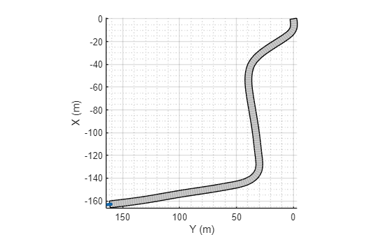
scenario = drivingScenario('GeoReference',origin);

Create a road based on the Cartesian coordinates of the route.

roadCenters = [xEast,yNorth,zUp];
road(scenario,roadCenters);

Create a vehicle that follows the center line of the road. The vehicle travels between 4 and 5 meters per second (9 to 11 miles per hour), slowing down at the curves in the road. To create the trajectory, use the smoothTrajectory function. The computed trajectory minimizes jerk and avoids discontinuities in acceleration, which is a requirement for modeling INS sensors.

egoVehicle = vehicle(scenario,'ClassID',1);
egoPath = roadCenters;
egoSpeed = [5 5 5 4 4 4 5 4 4 4 4 5 5 5 5 5];
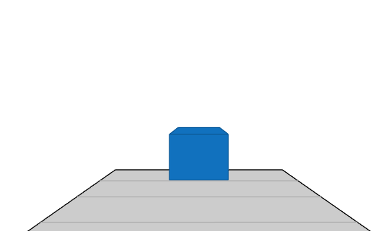
smoothTrajectory(egoVehicle,egoPath,egoSpeed);

Plot the scenario and show a 3-D view from behind the ego vehicle.

plot(scenario)

Figure contains an axes object. The axes object with xlabel X (m), ylabel Y (m) contains 3 objects of type patch, line.

chasePlot(egoVehicle)

Create INS Sensor

Create an INS sensor that accepts the input of simulation times. Introduce noise into the sensor measurements by setting the standard deviation of velocity and accuracy measurements to 0.1 and 0.05, respectively.

INS = insSensor('TimeInput',true, ...
                'VelocityAccuracy',0.1, ...
                'AccelerationAccuracy',0.05);

Visualize INS Measurements

Initialize a geographic player for displaying the INS measurements and the actor ground truth. Configure the player to display its last 10 positions and set the zoom level to 17.

zoomLevel = 17;
player = geoplayer(latIn(1),lonIn(1),zoomLevel, ...
    'HistoryDepth',10,'HistoryStyle','line');

Figure Geographic Player contains an axes object with type geoaxes. The geoaxes object is empty.

Pre-allocate space for the simulation times, velocity measurements, and acceleration measurements that are captured during simulation.

numWaypoints = length(latIn);
times = zeros(numWaypoints,1);
gTruthVelocities = zeros(numWaypoints,1);
gTruthAccelerations = zeros(numWaypoints,1);
sensorVelocities = zeros(numWaypoints,1);
sensorAccelerations = zeros(numWaypoints,1);

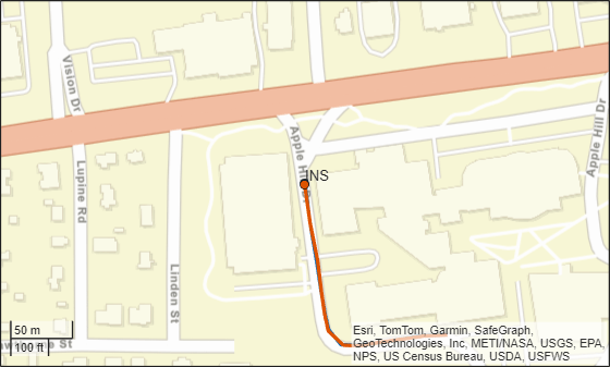
Simulate the scenario. During the simulation loop, obtain the ground truth state of the ego vehicle and an INS measurement of that state. Convert these readings to geographic coordinates, and at each waypoint, visualize the ground truth and INS readings on the geographic player. Also capture the velocity and acceleration data for plotting the velocity and acceleration profiles.

nextWaypoint = 2;
while advance(scenario)

    % Obtain ground truth state of ego vehicle.
    gTruth = state(egoVehicle);

    % Obtain INS sensor measurement.
    measurement = INS(gTruth,scenario.SimulationTime);

    % Convert readings to geographic coordinates.
    [latOut,lonOut] = local2latlon(measurement.Position(1), ...
                                   measurement.Position(2), ...
                                   measurement.Position(3),origin);

    % Plot differences between ground truth locations and locations reported by sensor.
    reachedWaypoint = sum(abs(roadCenters(nextWaypoint,:) - gTruth.Position)) < 1;
    if reachedWaypoint
        plotPosition(player,latIn(nextWaypoint),lonIn(nextWaypoint),'TrackID',1)
        plotPosition(player,latOut,lonOut,'TrackID',2,'Label','INS')

        % Capture simulation times, velocities, and accelerations.
        times(nextWaypoint,1) = scenario.SimulationTime;
        gTruthVelocities(nextWaypoint,1) = gTruth.Velocity(2);
        gTruthAccelerations(nextWaypoint,1) = gTruth.Acceleration(2);
        sensorVelocities(nextWaypoint,1) = measurement.Velocity(2);
        sensorAccelerations(nextWaypoint,1) = measurement.Acceleration(2);

        nextWaypoint = nextWaypoint + 1;
    end

    if nextWaypoint > numWaypoints
        break
    end

end

Figure contains an axes object. The axes object with xlabel X (m), ylabel Y (m) contains 3 objects of type patch, line.

Figure Geographic Player contains an axes object with type geoaxes. The geoaxes object contains 6 objects of type line, text.

Plot Velocity Profile

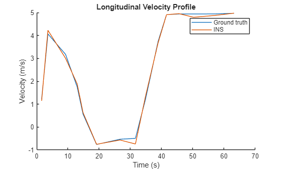
Compare the ground truth longitudinal velocity of the vehicle over time against the velocity measurements captured by the INS sensor.

Remove zeros from the time vector and velocity vectors.

times(times == 0) = [];
gTruthVelocities(gTruthVelocities == 0) = [];
sensorVelocities(sensorVelocities == 0) = [];

figure
hold on
plot(times,gTruthVelocities)
plot(times,sensorVelocities)
title('Longitudinal Velocity Profile')
xlabel('Time (s)')
ylabel('Velocity (m/s)')
legend('Ground truth','INS')
hold off

Figure contains an axes object. The axes object with title Longitudinal Velocity Profile, xlabel Time (s), ylabel Velocity (m/s) contains 2 objects of type line. These objects represent Ground truth, INS.

Plot Acceleration Profile

Compare the ground truth longitudinal acceleration of the vehicle over time against the acceleration measurements captured by the INS sensor.

gTruthAccelerations(gTruthAccelerations == 0) = [];
sensorAccelerations(sensorAccelerations == 0) = [];

figure
hold on
plot(times,gTruthAccelerations)
plot(times,sensorAccelerations)
title('Longitudinal Acceleration Profile')
xlabel('Time (s)')
ylabel('Acceleration (m/s^2)')
legend('Ground truth','INS')
hold off

Figure contains an axes object. The axes object with title Longitudinal Acceleration Profile, xlabel Time (s), ylabel Acceleration (m/s toThePowerOf 2) baseline contains 2 objects of type line. These objects represent Ground truth, INS.

Tips

  • To obtain the ground-truth state of actors in a driving scenario, use the state function.

  • The sensor reports measurements in the local Cartesian coordinate system. To convert these measurements to geographic positions for visualization on a map, use the local2latlon function. To convert this data back to local coordinates, use the latlon2local function.

Extended Capabilities

Version History

Introduced in R2021a