Generate RoadRunner Scene Using Labeled Camera Images and GPS Data

This example shows how to generate a RoadRunner scene containing add or drop lanes with junctions using labeled camera images and GPS waypoints.

You can create a virtual scene from recorded sensor data that represents real-world roads and use it to perform safety assessments for automated driving applications.

By combining camera images and GPS data, you can accurately reconstruct a road scene that contains lane information and junctions. Camera images enable you to easily identify scene elements, such as lane markings and road boundaries, while GPS waypoints enable you to place these elements in the world coordinate system. Additionally, you can improve the labeling of lane boundaries in images by using a variety of lane detectors that perform reliably regardless of the camera used. This example fuses lane boundary labels from images with GPS waypoints to generate an accurate scene.

In this example, you:

• Load a sequence of lane boundary-labeled images and GPS waypoints.

• Divide the scene into segments, with a fixed number of lane boundaries in each segment.

• Map the lane boundary labels across the entire sequence.

• Extract the lane boundary points from the images and transform them into the world coordinate system.

• Generate a RoadRunner HD Map from the extracted lane boundary points.

The workflow in this example requires labeled camera images, camera parameters and GPS waypoints.

Load Sensor Data and Lane Boundary Labels

This example requires the Scenario Builder for Automated Driving Toolbox™ support package. Check if the support package is installed and, if it is not installed, install it using the Get and Manage Add-Ons.

checkIfScenarioBuilderIsInstalled

Download a ZIP file containing a subset of sensor data from the PandaSet data set, and then unzip the file. This file contains data for a continuous sequence of 160 point clouds and images. The data also contains lane boundary labels in the form of pixel coordinates. The data stores these labels as a groundTruthMultisignal object. Alternatively, you can obtain lane boundary labels using a lane boundary detector. For more information, see Extract Lane Information from Recorded Camera Data for Scene Generation.

dataFolder = tempdir;
dataFilename = "PandasetSceneGeneration.zip";
url = "https://ssd.mathworks.com/supportfiles/driving/data/" + dataFilename;
filePath = fullfile(dataFolder,dataFilename);
if ~isfile(filePath)
    websave(filePath,url)
end
unzip(filePath,dataFolder)
dataset = fullfile(dataFolder,"PandasetSceneGeneration");

Load the downloaded data set into the workspace using the helperLoadData function.

[imds,~,sensor,gTruth,~,gps,timestamps] = helperLoadExampleData(dataset);

The output arguments of the helperLoadData function contains:

• imds — Datastore for images, specified as a imageDatastore object.

• sensor — Camera parameters, specified as a monoCamera object.

• gTruth — Lane boundary labels in pixel coordinate, specified as a groundTruthMultisignal object.

• gps — GPS coordinates of the ego vehicle, specified as a structure.

• timestamps — Time of capture, in seconds, for the lidar, camera, and GPS data.

Read the first point cloud, the first image, and its corresponding lane boundary labels.

img = read(imds);
boundaries = gTruth.ROILabelData.Camera{1,:}{1};

Overlay the lane boundary labels onto the image and visualize it.

figure
imshow(img)
hold on

for i = 1:length(boundaries)
    boundary = boundaries(i);
    points = boundary.Position;
    plot(points(:,1),points(:,2),LineWidth=3,Color="r")
end

hold off

Note: You can view the labels for all timestamps using the Ground Truth Labeler app by importing gTruth from the workspace or by calling groundTruthLabeler(gTruth).

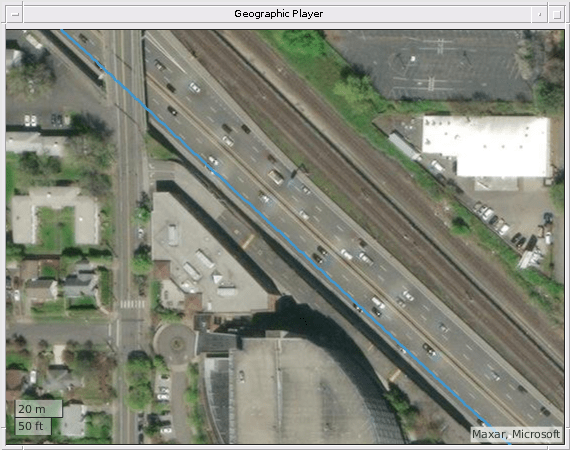
Visualize geographic map data with GPS trajectory of ego vehicle by using the helperPlotGPS function. Note that, in the figure the ego vehicle is moving from bottom-right to the top-left on the trajectory.

helperPlotGPS(gps);

Divide Scene into Segments with Fixed Number of Lane Boundaries

Divide the scene into smaller segments, each with a fixed number of lane boundaries by using the helperCreateSegments function. Dividing the scene into segments makes it easier to extract geometry of each lane boundary.

The helperCreateSegments function creates subsequent continuous segments with unique number of lane boundaries based on a specified threshold. In the sequence, when there are unequal lane boundaries, a segment is combined with the one before it if the ego vehicle's segmental travel distance is less than the specified threshold distance. Unit of threshold distance is in meters. The returned segments is an M-by-2 array specifying M number of road segments. For each row, the first and second column specifies the start and end indices of a road segment.

% Convert GPS waypoints to Cartesian coordinates
lat = [gps.lat]';
lon = [gps.long]';
alt = [gps.height]';
geoRef = [lat(1),lon(1),alt(1)];
[x,y,z] = latlon2local(lat,lon,alt,geoRef);
waypoints = [x,y,z];

% Divide the scene into segments
segments = helperCreateSegments(gTruth,waypoints,Threshold=18);

Visualize the obtained five segments by using the helperPlotGPS function.

helperPlotGPS(gps,segments);

Map Lane Boundaries

In a road segment, lane boundary labels may be missing for a few frames due to the lane boundary being occluded or moving out of the camera field-of-view. For example, in the image on the right, you can observe that as the ego-vehicle gets closer to the junction, the left-most lane boundaries move outside the camera field-of-view. To extract the points for each lane boundary for the entire sequence, you must map the two visible lane boundaries in the image on the right with the two right-most lane boundaries in the image on the left.

Map the lane boundaries in each frame with the lane boundaries in the previous frame by using the helperMapLaneLabels function. The function returns an M-by-1 cell array, specifying lane b

oundaries for M segments. For each cell entry, the lane boundaries are sorted in left-to-right order.

mappedBoundaries = cell(size(segments,1),1);
for i = 1:size(segments,1)
    mappedBoundaries{i} = helperMapLaneBoundaryLabels(gTruth,sensor,segments(i,:));
end

Plot the mapped lane boundaries for a frame by using the helperPlotLaneBoundaries function. This function displays the lane boundaries numbered from left to right.

segmentNumber = 2;
frameNumber = 45;
helperPlotLaneBoundaries(imds,mappedBoundaries,segments,segmentNumber,frameNumber);
title("All Lane Boundaries Visible")

Plot the lane boundaries for a subsequent frame. In this figure, you observe that the two right-most lane boundaries are numbered 3 and 4 even after the other boundaries move out of the camera field-of-view.

segmentNumber = 2;
frameNumber = 52;
helperPlotLaneBoundaries(imds,mappedBoundaries,segments,segmentNumber,frameNumber);
title("Only Right Lane Boundaries Visible")

Extract Lane Geometry from Lane Boundary Labels and GPS Trajectory

Use the helperConvertImageToVehicle function to convert the lane boundary points from image pixel locations to the vehicle coordinate system by using a projective transformation.

mappedBoundaries = helperConvertImageToVehicle(mappedBoundaries,sensor);

Note that these issues may result in inaccurate lane boundary points:

• Camera lens distortion — This affects the accuracy of image pixel coordinates, because of which the obtained lane boundaries may appear warped or curved. If your image data contains distortion, you can correct them by using the undistortPoints function.

• Road surface condition — This affects the positional accuracy of lane boundary points in pixel coordinates. For example, if the road has dips or bumps, the camera's viewpoint may change, leading to inaccurate lane boundary points. If your test road surface is not flat, you can combine lidar data with camera data to get accurate lane boundary points. For more information, see Generate RoadRunner Scene Using Labeled Camera Images and Raw Lidar Data.

Calculate the yaw angles of the ego-vehicle for each timestamp using the GPS or IMU data. In this example, yaw angles are calculated using the GPS waypoints. Note that the GPS waypoints used in this example are from a highly accurate sensor. Orientations obtained using this method may be inaccurate for noisy GPS data. If IMU data is available, you can fuse with the GPS data to accurately estimate ego-vehicle position and orientation. For more information, see Ego Vehicle Localization Using GPS and IMU Fusion for Scenario Generation.

yaw = atan2(y(2:end)-y(1:end-1),x(2:end)-x(1:end-1));
yaw = [yaw;yaw(end)];

Create an array of ego-vehicle to the world coordinate system rigid transformations with reference to the ego position and yaw information.

tforms = [];
for i = 1:size(waypoints,1)
    tform = rigidtform2d(rad2deg(yaw(i)),[x(i) y(i)]);
    tforms = [tforms;tform];
end

Transform the mapped lane boundaries from vehicle coordinate system to the world coordinate system using the computed transformations.

laneBoundaryPoints = cell(size(segments,1),1);
for j = 1:size(segments,1)
    % Create a container for lane boundary points of current segment
    segmentPoints = cell(1,size(mappedBoundaries{j},2));
    % Get lane boundary points for current segment
    boundaries = mappedBoundaries{j};
    for i = segments(j,1):segments(j,2)
        % Create a container for lane boundary points of current frame
        lanes = mappedBoundaries{j}(i-segments(j,1)+1,:);
        % Loop over all the lane boundaries and transform the points
        for k = 1:length(lanes)
            points = lanes{k};
            if ~isempty(points)
                % Apply forward geometric transformation to the lane boundarie points
                [xT,yT] = transformPointsForward(tforms(i),points(:,1),points(:,2));
                segmentPoints{k} = [segmentPoints{k};[xT,yT]];
            end
        end
    end
    % Update the transformed lane boundary points
    laneBoundaryPoints{j} = segmentPoints;
end

Visualize the transformed lane boundary points in the world coordinate system.

figure
hold on
for i = 1:length(laneBoundaryPoints)
    for j = 1:length(laneBoundaryPoints{i})
        if ~isempty(laneBoundaryPoints{i}{1})
            plot(laneBoundaryPoints{i}{j}(:,1),laneBoundaryPoints{i}{j}(:,2),"b.")
        end
    end
end
title("Lane Boundary Points in World Coordinate System")
hold off

Use the helperSortPointsInTravelDirection function to sort the extracted lane boundary points along the travel direction. This is necessary to ensure that the geometries of the road segments are connected correctly. The function computes the ego-vehicle travel directions by comparing the start and end x-coordinates of the ego-vehicle waypoints.

laneBoundaryPoints = helperSortPointsInTravelDirection(laneBoundaryPoints,waypoints,segments);

Create RoadRunner HD Map

Create a RoadRunner HD Map from the extracted lane boundary points by using the roadrunnerLaneInfo function. This function automatically connects the geometry of consecutive road segments. Specify the MinJunctionLength argument as 10 to automatically insert a perpendicular road at the junction.

% Delete the empty segments
empty_idx = cellfun(@(x) isempty(x{1}),laneBoundaryPoints);
laneBoundaryPoints(empty_idx) = [];

% Create a RoadRunner HD Map
rrMap = roadrunnerHDMap;
[laneInfo,geographicBoundary] = roadrunnerLaneInfo(laneBoundaryPoints,SmoothingDegree=1,SmoothingFactor=0.25,MinJunctionLength=10);
rrMap.Lanes = laneInfo.Lanes;
rrMap.LaneBoundaries = laneInfo.LaneBoundaries;
rrMap.GeographicBoundary = geographicBoundary;
write(rrMap,"rrMap.rrhd")

Visualize the generated RoadRunner HD Map along with the ego-vehicle waypoints.

plot(rrMap)
hold on
plot(waypoints(:,1),waypoints(:,2),"bo")
legend("Lane Boundaries","Lane Centers","Ego-Vehicle Waypoints")

Write the RoadRunner HD Map to a binary file, which you can import into RoadRunner.

write(rrMap,"rrMap.rrhd")

To open RoadRunner using MATLAB®, specify the path to your RoadRunner project. This code shows the path for a sample project folder location in Windows®.

rrProjectPath = "C:\RR\MyProject";

Specify the path to your local RoadRunner installation folder. This code shows the path for the default installation location in Windows.

rrAppPath = "C:\Program Files\RoadRunner R2023a\bin\win64";

Open RoadRunner using the specified path to your project.

rrApp = roadrunner(rrProjectPath,InstallationFolder=rrAppPath);

Specify the RoadRunner HD Map import options. Set the enableOverlapGroupsOptions to false to ensure that a junction is built at the two intersecting roads.

overlapGroupsOptions = enableOverlapGroupsOptions(IsEnabled=false);
buildOptions = roadrunnerHDMapBuildOptions(EnableOverlapGroupsOptions=overlapGroupsOptions);
importOptions = roadrunnerHDMapImportOptions(BuildOptions=buildOptions);

Import the rrMap.rrhd scene into RoadRunner.

importScene(rrApp,fullfile(pwd,"rrMap.rrhd"),"RoadRunner HD Map",importOptions);

Use Lane Marking Tool to mark lane boundaries in the imported road. This figure shows the built road in RoadRunner that contains a junction with add and drop lanes.

Note: Use of the Scene Builder Tool requires a RoadRunner Scene Builder license.