Ego Vehicle Localization Using GPS and IMU Fusion for Scenario Generation
This example shows how to perform ego vehicle localization by fusing global positioning system (GPS) and inertial measurement unit (IMU) sensor data for creating a virtual scenario.
Using recorded vehicle data, you can generate virtual driving scenarios to recreate a real-world scenario. Virtual scenarios enable you to study and visualize these recorded scenarios. To generate a reliable virtual scenario, you must have accurate ego vehicle localization data, which consists of position and orientation information.
GPS sensors can indicate the position of the vehicle, but orientation information is not always available. Further, GPS data often suffers from noise and bias. So, if you estimate orientation using GPS data, you can get inaccurate results. IMU sensors such as accelerometers and gyroscopes are less prone to noise but can only provide relative information (that is, the acceleration and angular velocity) about the movement of the ego vehicle. This example shows how to perform information fusion using GPS and IMU sensor data to accurately estimate both the position and orientation of the ego vehicle. You then use this accurate ego trajectory to create a RoadRunner scenario. If the trajectory contains drift, see Ego Localization Using Lane Detections and HD Map for Scenario Generation example to correct that.
Load Recorded Sensor Data
This example requires the Scenario Builder for Automated Driving Toolbox™ support package. Check if the support package is installed and, if it is not installed, install it using the Get and Manage Add-Ons.
checkIfScenarioBuilderIsInstalled
Download a ZIP file containing a subset of the Comma2k19 data set [1], and then unzip the file. This file contains recorded data from camera, GPS, and IMU sensors and ground truth information on the ego trajectory. In this example, you use the camera data for visual validation of the generated scenario.
dataFolder = tempdir;
dataFilename = "CommaData.zip";
url = "https://ssd.mathworks.com/supportfiles/driving/data/"+dataFilename;
filePath = fullfile(dataFolder,dataFilename);
if ~isfile(filePath)
    websave(filePath,url);
end
unzip(filePath,dataFolder)
Load the GPS data into the workspace.
dataset = fullfile(dataFolder,"CommaData");
data = load(fullfile(dataset,"sensorData"+filesep+"gps.mat"));
gpsData = data.gpsData;
gpsData is a table with these columns:
timeStamp— Time, in seconds, at which the GPS data was collected.latitude— Latitude coordinate value of the ego vehicle. Units are in degrees.longitude— Longitude coordinate value of the ego vehicle. Units are in degrees.altitude— Altitude coordinate value of the ego vehicle. Units are in meters.
Extract GPS data from the recorded GPS readings and load them in the workspace.
gpsTimestamps = gpsData.timeStamp;
latitude = gpsData.latitude;
longitude = gpsData.longitude;
altitude = gpsData.altitude;
Create a GPSData object by using the recordedSensorData function to store the loaded GPS data.
gpsData = recordedSensorData("gps",gpsTimestamps,latitude,longitude,altitude)gpsData =
GPSData with properties:
Name: ''
NumSamples: 308
Duration: 59.8003
SampleRate: 5.1505
SampleTime: 0.1948
Timestamps: [308×1 double]
Latitude: [308×1 double]
Longitude: [308×1 double]
Altitude: [308×1 double]
Attributes: []
Visualize the GPS path of the ego vehicle by using the plot object function.
plot(gpsData,"ZoomLevel",14,"MarkerSize",3)
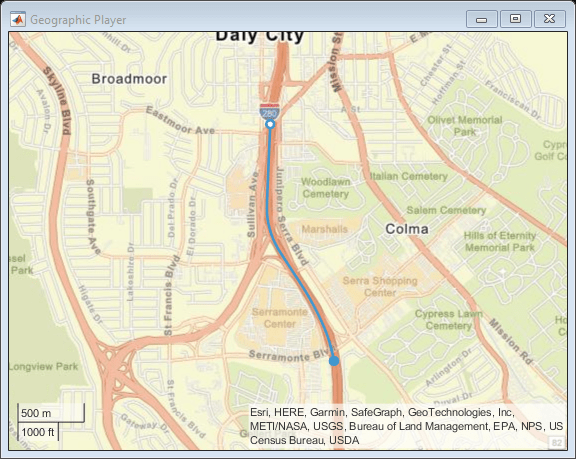
Load the IMU data into the workspace. The data contains the linear acceleration values recorded using an accelerometer and angular velocity values recorded using gyroscope sensors. This data is in the North-East-Down (NED) reference frame.
data = load(fullfile(dataset,"sensorData"+filesep+"imu.mat"));
imuData = data.imuData;
imuData is a table with these columns:
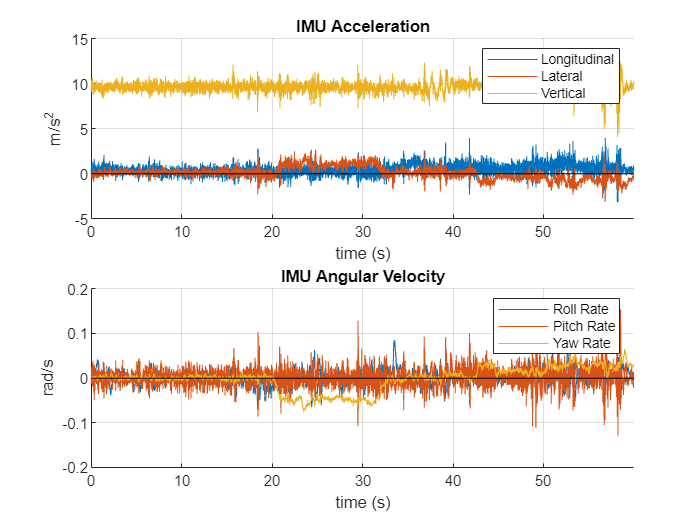
timeStamp— Time, in seconds, at which the IMU data was collected.longitudinalAcceleration— Longitudinal component of linear acceleration of the ego vehicle. Units are in meters per second squared.lateralAcceleration— Lateral component of the linear acceleration of the ego vehicle. Units are in meters per second squared.verticalAcceleration— Vertical component of the linear acceleration of the ego vehicle. Units are in meters per second squared.rollRate— Roll rate component of the angular velocity of the ego vehicle. Units are in radians per second.pitchRate— Pitch rate component of the angular velocity of the ego vehicle. Units are in radians per second.yawRate— Yaw rate component of the angular velocity of the ego vehicle. Units are in radians per second.
Plot the IMU data using the helperPlotIMUData function.
helperPlotIMUData(imuData)
To fuse GPS and IMU data, this example uses an extended Kalman filter (EKF) and tunes the filter parameters to get the optimal result. You use ground truth information, which is given in the Comma2k19 data set and obtained by the procedure as described in [1], to initialize and tune the filter parameters.
Load the ground truth data, which is in the NED reference frame, into the workspace.
data = load(fullfile(dataset,"groundTruthData"+filesep+"groundTruth.mat"));
groundTruthData = data.groundTruthData;
groundTruthData is a table with these columns:
timeStamp— Time, in seconds, at which the ground truth data was collected.position— Ground truth positions of the ego vehicle. Units are in meters.orientation— Ground truth orientations of the ego vehicle in the [yaw,pitch,roll] format. Units are in radians.
Preprocess Data
Get GPS latitude, longitude, and altitude data.
gpsLLA = [gpsData.Latitude gpsData.Longitude gpsData.Altitude];
Convert the GPS data into timetable format because the filter and tuner support this format.
gpsTT = timetable(seconds(gpsData.Timestamps),gpsLLA);
gpsTT.Properties.VariableNames(1) = "GPS";
Get the linear acceleration and angular velocity data from the IMU sensor.
acceleration = [imuData.longitudinalAcceleration imuData.lateralAcceleration imuData.verticalAcceleration];
angularVelocity = [imuData.rollRate imuData.pitchRate imuData.yawRate];
Convert the IMU data into timetable format because the filter and tuner support this format.
imuData = timetable(seconds(imuData.timeStamp),acceleration,angularVelocity);
imuData.Properties.VariableNames(1) = "Accelerometer";
imuData.Properties.VariableNames(2) = "Gyroscope";
Get the ground truth positions of the ego vehicle.
gtPosition = groundTruthData.position;
Get the ground truth orientations of the ego vehicle.
gtOrientation = quaternion(groundTruthData.orientation,"euler","ZYX","frame");
A quaternion and its negative represent the same orientation. Find quaternions with a nonnegative real part and invert them using the helperConvertQuatPositive function for better tuner convergence.
gtOrientation = helperConvertQuatPositive(gtOrientation);
Convert the ground truth data into timetable format.
groundTruthData = timetable(seconds(groundTruthData.timeStamp),gtOrientation,gtPosition);
groundTruthData.Properties.VariableNames(1) = "Orientation";
groundTruthData.Properties.VariableNames(2) = "Position";
Synchronize the ground truth and sensor data using the helperSyncGPSIMUWithGroundTruth function. The function also cleans up ground truth data by removing rows that contain NaN values. You use these synchronized data to tune the filter.
[sensorData,groundTruthData] = helperSyncGPSIMUWithGroundTruth(gpsTT,imuData,groundTruthData);
Normalize the timestamps of the sensor and ground truth data.
startTime = sensorData.Time(1);
sensorData.Time = sensorData.Time - startTime;
groundTruthData.Time = groundTruthData.Time - startTime;
Display the first five entries of sensor data. Because the sampling rate of GPS data is less than that of IMU data, GPS data is not available at all timestamps. The table represents missing GPS data using NaN values.
sensorData(1:5,:)
ans=5×3 timetable
        Time                  Accelerometer                              Gyroscope                               GPS
    ____________    __________________________________    _______________________________________    ____________________________

    0 sec           -0.11725     0.014359       9.1286    -0.003006      -0.013123      0.0018005       NaN        NaN        NaN
    0.050007 sec     0.54796     -0.26561        9.131    0.0043182      0.0076447     0.00059509       NaN        NaN        NaN
    0.10002 sec       1.0504    -0.033493       9.7603    0.0031128       0.024765     0.00059509       NaN        NaN        NaN
    0.15002 sec      0.93559    0.0071716       10.047     0.014099       0.014969     -0.0018463    37.685    -122.47     23.824
    0.20001 sec      0.10768     -0.10049       9.9757     0.023865       0.011322    -0.00064087       NaN        NaN        NaN
Display the first five entries of ground truth data.
groundTruthData(1:5,:)
ans=5×2 timetable
        Time         Orientation                  Position
    ____________    ______________    _________________________________

    0 sec           1×1 quaternion          0            0            0
    0.050007 sec    1×1 quaternion    -1.4219    -0.071088     0.057686
    0.10002 sec     1×1 quaternion    -2.8477       -0.141      0.11388
    0.15002 sec     1×1 quaternion    -4.2755     -0.21034      0.16785
    0.20001 sec     1×1 quaternion    -5.7056     -0.27938      0.21915
GPS and IMU Sensor Data Fusion
This example uses an extended Kalman filter (EKF) to asynchronously fuse GPS, accelerometer, and gyroscope data using an insEKF (Sensor Fusion and Tracking Toolbox) object. Create sensor models for the accelerometer, gyroscope, and GPS sensors.
hacc = insAccelerometer;
hgyro = insGyroscope;
hgps = insGPS;
To set the reference location for the GPS sensor model, use the GPS data corresponding to the first ground truth position data point. Because GPS data is not available at all timestamps, find the timestamp corresponding to the first valid (non-NaN) point of GPS data. Then, for that timestamp, get the ground truth position data. Use this value as the origin of the local NED coordinate system to estimate the GPS value for the first ground truth position.
firstNonNANGPSPosition = find(~isnan(sensorData.GPS),1,"first");
refLoc = ned2lla(groundTruthData.Position(1,:) - groundTruthData.Position(firstNonNANGPSPosition,:),sensorData.GPS(firstNonNANGPSPosition,:),"ellipsoid");
hgps.ReferenceLocation = refLoc;
If you do not have ground truth data, estimate the reference location using one of these options:
Find the mean of first few GPS data points.
If you have GPS data from when the vehicle is stationary, find the mean of the GPS data points for those timestamps.
Create an insEKF object using the sensor models.
filter = insEKF(hacc,hgyro,hgps)
filter =
  insEKF with properties:

                   State: [22×1 double]
         StateCovariance: [22×22 double]
    AdditiveProcessNoise: [22×22 double]
             MotionModel: [1×1 insMotionPose]
                 Sensors: {[1×1 insAccelerometer]  [1×1 insGyroscope]  [1×1 insGPS]}
             SensorNames: {'Accelerometer'  'Gyroscope'  'GPS'}
          ReferenceFrame: 'NED'
Initialize the position part of the state in the filter using the first ground truth position data. Initialize the diagonal elements of the state estimate error covariance matrix corresponding to the position state.
stateparts(filter,Position=groundTruthData.Position(1,:));
statecovparts(filter,Position=1e-7);
If you do not have ground truth data, initialize the position part of the state in the filter using the GPS measurement data. Convert the first few GPS measurements to local Cartesian coordinates using the latlon2local function with the reference location and compute the mean of the output coordinates. If you adapt this example to your own application and are uncertain about the accuracy of the data used for initialization, then set the state estimates of the error covariance matrix to higher values than those used in this example.
Initialize the velocity part of the state in the filter using the time and position data. To get a robust estimate, this example finds the mean of the first 10 velocity values.
diffTime = mean(diff(seconds(groundTruthData.Time)));
vtmp = diff(groundTruthData.Position)./diffTime;
vinit = mean(vtmp(1:10,:));
stateparts(filter,Velocity=vinit);
Initialize the acceleration part of the state in the filter using the time and velocity data. To get the robust estimate, this example finds the mean of first 10 acceleration values.
atmp = diff(vtmp)./diffTime;
ainit = mean(atmp(1:10,:));
stateparts(filter,Acceleration=ainit);
Initialize the orientation part of the state in the filter. To get a robust estimate, this example finds the mean of the first 10 ground truth values.
qinit = meanrot(groundTruthData.Orientation(1:10));
stateparts(filter,Orientation=compact(qinit));
statecovparts(filter,Orientation=1e-5);
If you do not have ground truth data, then you can use the helperEstimateOrientation function to estimate initial orientation state from the sensor data. The function estimates the initial orientation from the velocities estimated using sensor data, for example, qinit = helperEstimateOrientation(velocities).
Because the gyroscope readings are in the sensor frame and the state estimates are required in the navigation frame, convert the first gyroscope measurement from sensor frame to navigation frame and use it to initialize the angular velocity part of the state in the filter.
avinit = rotatepoint(qinit,sensorData.Gyroscope(1,:));
stateparts(filter,AngularVelocity=avinit);
statecovparts(filter,AngularVelocity=1e-3);
To reduce the estimation error between the fused sensor data and ground truth, tune the parameters of the insEKF filter using the helperTuneInsEKF function. The function finds the optimal values of measurement noise and additive process noise for the filter. For more information on tuning an insEKF filter, see tune (Sensor Fusion and Tracking Toolbox).
[tunedFilter,tunedMeasureNoise] = helperTuneInsEKF(filter,sensorData,groundTruthData);
If you do not have ground truth data, then you need to manually tune these parameters for optimal performance.
Since you have batch data, you can use smoothing. Perform batch fusion of the sensor data using the estimateStates (Sensor Fusion and Tracking Toolbox) function, which returns smoothed state estimates.
[~,sm] = estimateStates(tunedFilter,sensorData,tunedMeasureNoise);
Extract the fused position, orientation, and time information from the smoothed state estimates.
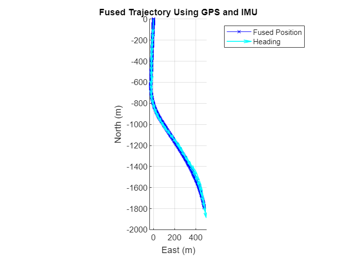
fusedPosition= sm.Position;
fusedOrientation= sm.Orientation;
fusedTime = seconds(sm.Time);
Visualize the fused position and heading direction using the helperPlotHeadingAndPosition function.
helperPlotHeadingAndPosition(fusedPosition,fusedOrientation,30);
Generate RoadRunner Scenario
Generate a RoadRunner scenario to visualize the ego vehicle trajectory after GPS and IMU sensor data fusion. RoadRunner requires the position and orientation data in the East-North-Up (ENU) reference frame. Convert the fused position and orientation data from NED to ENU reference frame using the helperConvertNED2ENU function.
[fusedPositionENU,fusedOrientationENU] = helperConvertNED2ENU(fusedPosition,fusedOrientation);
Add the altitude component of the reference location used in the insEKF filter to the altitude component of fused positions and get the absolute altitudes for the fused ego trajectory.
fusedPositionENU(:,3) = fusedPositionENU(:,3) + refLoc(3);
Create a Trajectory object by using the recordedSensorData function from fused position and fused orientation.
fusedTrajectoy = recordedSensorData("trajectory",fusedTime,fusedPositionENU,Orientation=quat2eul(fusedOrientationENU,"ZYX"))
fusedTrajectoy =
  Trajectory with properties:

               Name: ''

         NumSamples: 1200
           Duration: 59.9492
         SampleRate: 20.0170
         SampleTime: 0.0500
         Timestamps: [1200×1 double]

           Position: [1200×3 double]
        Orientation: [1200×3 double]
           Velocity: [1200×3 double]
             Course: [1200×1 double]
        GroundSpeed: [1200×1 double]
       Acceleration: [1200×3 double]
    AngularVelocity: [1200×3 double]

        LocalOrigin: [0 0 0]
         TimeOrigin: 0

         Attributes: []
Visualize the trajectory by using the plot object function.
plot(fusedTrajectoy,ShowHeading=true,ShowOrientation=true,ShowVelocity=true);

To find the accuracy of the fused trajectory by sensor fusion, you must compare it with the raw trajectory. Extract the raw vehicle trajectory from GPS coordinates by using the trajectory object function.
gpsTrajectory = trajectory(gpsData,"LocalOrigin",refLoc)gpsTrajectory =
Trajectory with properties:
Name: ''
NumSamples: 308
Duration: 59.8003
SampleRate: 5.1505
SampleTime: 0.1948
Timestamps: [308×1 double]
Position: [308×3 double]
Orientation: [308×3 double]
Velocity: [308×3 double]
Course: [308×1 double]
GroundSpeed: [308×1 double]
Acceleration: [308×3 double]
AngularVelocity: [308×3 double]
LocalOrigin: [37.6852 -122.4715 23.9918]
TimeOrigin: 3.7509e+03
Attributes: []
To open RoadRunner using MATLAB®, specify the path to your local RoadRunner installation folder. This code shows the path for the default installation location in Windows®.
rrAppPath = "C:\Program Files\RoadRunner R2024b\bin\win64";Specify the path to your RoadRunner project. This code shows the path to a sample project folder on Windows.
rrProjectPath = "C:\RR\MyProjects";Open RoadRunner using the specified path to your project.
rrApp = roadrunner(rrProjectPath,InstallationFolder=rrAppPath);
Export the trajectories into RoadRunner by using the exportToRoadRunner object function. Specify the file name of the RoadRunner scene, name, and color for the actor in RoadRunner. This example uses a RoadRunner scene created from Comma2k19 data set [1], attached to this example as a supporting file. The geographic coordinates of the scene origin are set to the local origin of the trajectory. For more information on creating a RoadRunner scene from the camera data, see the Generate RoadRunner Scene Using Processed Camera Data and GPS Data example.
sceneName = "commaScene.rrscene";
if ~isfile(sceneName)
    copyfile(sceneName,fullfile(rrProjectPath,"Scenes"));
end
exportToRoadRunner(fusedTrajectoy,rrApp,RoadRunnerScene=sceneName,Name="Fused",Color="white")
ans =
  roadrunner with properties:

    InstallationFolder: 'C:\Program Files\RoadRunner R2024b\bin\win64'
               Version: "R2024b Update 5 (1.9.5.0b7c32ffebc)"
             NoDisplay: 0
exportToRoadRunner(gpsTrajectory,rrApp,Name="RawGPS",Color="red",SetupSimulation=false)
ans =
  roadrunner with properties:

    InstallationFolder: 'C:\Program Files\RoadRunner R2024b\bin\win64'
               Version: "R2024b Update 5 (1.9.5.0b7c32ffebc)"
             NoDisplay: 0
rrSim = createSimulation(rrApp);
endTime = fusedTime(end);
set(rrSim,MaxSimulationTime=endTime);
set(rrSim,StepSize=0.1);
set(rrSim,Logging="on");
Monitor the status of the simulation and wait for the simulation to complete. Because RoadRunner Scenario cannot remove actors after their exit times, scenario simulation can fail due to collision. To avoid stopping the scenario on collision, remove fail conditions using these steps:
1. In the Logic editor, click the condition node at the end of the scenario.
2. In the Attributes pane, click Remove Fail Condition.
set(rrSim,SimulationCommand="Start")
while strcmp(get(rrSim,"SimulationStatus"),"Running")
    simstatus = get(rrSim,'SimulationStatus');
    pause(1)
end
To view the scenario from the ego vehicle view or chase view, in the Simulation pane, in the Camera section, set Camera View to either Follow or Front. Then, set the Actor attribute to Fused, which is the ego vehicle following the fused trajectory for the scenario in this example.
This figure shows the recorded camera data and generated RoadRunner scenario. The red car in the RoadRunner scenario follows the raw GPS trajectory, which shows some instability and bias. The white car corrects the instability and bias in its motion by following the trajectory generated by fusing GPS and IMU sensor data.

References
[1] Schafer, Harald, Eder Santana, Andrew Haden, and Riccardo Biasini. “A Commute in Data: The Comma2k19 Dataset,” 2018. https://doi.org/10.48550/arXiv.1812.05752.
See Also
Functions
Objects
Topics
- Overview of Scenario Generation from Recorded Sensor Data
- Smooth GPS Waypoints for Ego Localization
- Ego Localization Using Lane Detections and HD Map for Scenario Generation
- Generate High Definition Scene from Lane Detections and OpenStreetMap
- Extract Vehicle Track List from Recorded Camera Data for Scenario Generation
- Generate Scenario from Actor Track Data and GPS Data