fitcecoc

Fit multiclass models for support vector machines or other classifiers

Syntax

Mdl = fitcecoc(Tbl,ResponseVarName)

Mdl = fitcecoc(Tbl,formula)

Mdl = fitcecoc(Tbl,Y)

Mdl = fitcecoc(X,Y)

Mdl = fitcecoc(___,Name,Value)

[Mdl,HyperparameterOptimizationResults] = fitcecoc(___,Name,Value)

Description

Mdl = fitcecoc(Tbl,ResponseVarName) returns a full, trained, multiclass, error-correcting output codes (ECOC) model using the predictors in table Tbl and the class labels in Tbl.ResponseVarName. fitcecoc uses K(K – 1)/2 binary support vector machine (SVM) models using the one-versus-one coding design, where K is the number of unique class labels (levels). Mdl is a ClassificationECOC model.

Mdl = fitcecoc(Tbl,formula) returns an ECOC model using the predictors in table Tbl and the class labels. formula is an explanatory model of the response and a subset of predictor variables in Tbl used for training.

Mdl = fitcecoc(Tbl,Y) returns an ECOC model using the predictors in table Tbl and the class labels in vector Y.

Mdl = fitcecoc(X,Y) returns a trained ECOC model using the predictors X and the class labels Y.

Mdl = fitcecoc(___,Name,Value) returns an ECOC model with additional options specified by one or more Name,Value pair arguments, using any of the previous syntaxes.

For example, specify different binary learners, a different coding design, or to cross-validate. It is good practice to cross-validate using the Kfold Name,Value pair argument. The cross-validation results determine how well the model generalizes.

[Mdl,HyperparameterOptimizationResults] = fitcecoc(___,Name,Value) also returns hyperparameter optimization details when you specify the OptimizeHyperparameters name-value pair argument and use linear or kernel binary learners. For other Learners, the HyperparameterOptimizationResults property of Mdl contains the results.

Examples

Train Multiclass Model Using SVM Learners

Train a multiclass error-correcting output codes (ECOC) model using support vector machine (SVM) binary learners.

Load Fisher's iris data set. Specify the predictor data X and the response data Y.

load fisheriris
X = meas;
Y = species;

Train a multiclass ECOC model using the default options.

Mdl = fitcecoc(X,Y)

Mdl = 
  ClassificationECOC
             ResponseName: 'Y'
    CategoricalPredictors: []
               ClassNames: {'setosa'  'versicolor'  'virginica'}
           ScoreTransform: 'none'
           BinaryLearners: {3x1 cell}
               CodingName: 'onevsone'


  Properties, Methods

Mdl is a ClassificationECOC model. By default, fitcecoc uses SVM binary learners and a one-versus-one coding design. You can access Mdl properties using dot notation.

Display the class names and the coding design matrix.

Mdl.ClassNames

ans = 3x1 cell
    {'setosa'    }
    {'versicolor'}
    {'virginica' }

CodingMat = Mdl.CodingMatrix

CodingMat = 3×3

     1     1     0
    -1     0     1
     0    -1    -1

A one-versus-one coding design for three classes yields three binary learners. The columns of CodingMat correspond to the learners, and the rows correspond to the classes. The class order is the same as the order in Mdl.ClassNames. For example, CodingMat(:,1) is [1; –1; 0] and indicates that the software trains the first SVM binary learner using all observations classified as 'setosa' and 'versicolor'. Because 'setosa' corresponds to 1, it is the positive class; 'versicolor' corresponds to –1, so it is the negative class.

You can access each binary learner using cell indexing and dot notation.

Mdl.BinaryLearners{1}   % The first binary learner

ans = 
  CompactClassificationSVM
             ResponseName: 'Y'
    CategoricalPredictors: []
               ClassNames: [-1 1]
           ScoreTransform: 'none'
                     Beta: [4x1 double]
                     Bias: 1.4492
         KernelParameters: [1x1 struct]


  Properties, Methods

Compute the resubstitution classification error.

error = resubLoss(Mdl)

error = 0.0067

The classification error on the training data is small, but the classifier might be an overfitted model. You can cross-validate the classifier using crossval and compute the cross-validation classification error instead.

Train Multiclass Linear Classification Model

Train an ECOC model composed of multiple binary, linear classification models.

Load the NLP data set.

load nlpdata

X is a sparse matrix of predictor data, and Y is a categorical vector of class labels. There are more than two classes in the data.

Create a default linear-classification-model template.

t = templateLinear();

To adjust the default values, see the Name-Value Pair Arguments on templateLinear page.

Train an ECOC model composed of multiple binary, linear classification models that can identify the product given the frequency distribution of words on a documentation web page. For faster training time, transpose the predictor data, and specify that observations correspond to columns.

X = X';
rng(1); % For reproducibility 
Mdl = fitcecoc(X,Y,'Learners',t,'ObservationsIn','columns')

Mdl = 
  CompactClassificationECOC
      ResponseName: 'Y'
        ClassNames: [comm    dsp    ecoder    fixedpoint    ...    ]
    ScoreTransform: 'none'
    BinaryLearners: {78x1 cell}
      CodingMatrix: [13x78 double]


  Properties, Methods

Alternatively, you can train an ECOC model composed of default linear classification models using 'Learners','Linear'.

To conserve memory, fitcecoc returns trained ECOC models composed of linear classification learners in CompactClassificationECOC model objects.

Cross-Validate ECOC Classifier

Cross-validate an ECOC classifier with SVM binary learners, and estimate the generalized classification error.

Load Fisher's iris data set. Specify the predictor data X and the response data Y.

load fisheriris
X = meas;
Y = species;
rng(1); % For reproducibility

Create an SVM template, and standardize the predictors.

t = templateSVM('Standardize',true)

t = 
Fit template for classification SVM.

                     Alpha: [0x1 double]
             BoxConstraint: []
                 CacheSize: []
             CachingMethod: ''
                ClipAlphas: []
    DeltaGradientTolerance: []
                   Epsilon: []
              GapTolerance: []
              KKTTolerance: []
            IterationLimit: []
            KernelFunction: ''
               KernelScale: []
              KernelOffset: []
     KernelPolynomialOrder: []
                  NumPrint: []
                        Nu: []
           OutlierFraction: []
          RemoveDuplicates: []
           ShrinkagePeriod: []
                    Solver: ''
           StandardizeData: 1
        SaveSupportVectors: []
            VerbosityLevel: []
                   Version: 2
                    Method: 'SVM'
                      Type: 'classification'

t is an SVM template. Most of the template object properties are empty. When training the ECOC classifier, the software sets the applicable properties to their default values.

Train the ECOC classifier, and specify the class order.

Mdl = fitcecoc(X,Y,'Learners',t,...
    'ClassNames',{'setosa','versicolor','virginica'});

Mdl is a ClassificationECOC classifier. You can access its properties using dot notation.

Cross-validate Mdl using 10-fold cross-validation.

CVMdl = crossval(Mdl);

CVMdl is a ClassificationPartitionedECOC cross-validated ECOC classifier.

Estimate the generalized classification error.

genError = kfoldLoss(CVMdl)

genError = 0.0400

The generalized classification error is 4%, which indicates that the ECOC classifier generalizes fairly well.

Estimate Posterior Probabilities Using ECOC Classifier

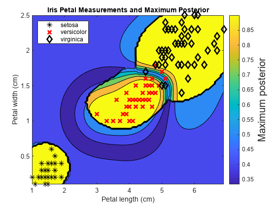
Train an ECOC classifier using SVM binary learners. First predict the training-sample labels and class posterior probabilities. Then predict the maximum class posterior probability at each point in a grid. Visualize the results.

Load Fisher's iris data set. Specify the petal dimensions as the predictors and the species names as the response.

load fisheriris
X = meas(:,3:4);
Y = species;
rng(1); % For reproducibility

Create an SVM template. Standardize the predictors, and specify the Gaussian kernel.

t = templateSVM('Standardize',true,'KernelFunction','gaussian');

t is an SVM template. Most of its properties are empty. When the software trains the ECOC classifier, it sets the applicable properties to their default values.

Train the ECOC classifier using the SVM template. Transform classification scores to class posterior probabilities (which are returned by predict or resubPredict) using the 'FitPosterior' name-value pair argument. Specify the class order using the 'ClassNames' name-value pair argument. Display diagnostic messages during training by using the 'Verbose' name-value pair argument.

Mdl = fitcecoc(X,Y,'Learners',t,'FitPosterior',true,...
    'ClassNames',{'setosa','versicolor','virginica'},...
    'Verbose',2);

Training binary learner 1 (SVM) out of 3 with 50 negative and 50 positive observations.
Negative class indices: 2
Positive class indices: 1

Fitting posterior probabilities for learner 1 (SVM).
Training binary learner 2 (SVM) out of 3 with 50 negative and 50 positive observations.
Negative class indices: 3
Positive class indices: 1

Fitting posterior probabilities for learner 2 (SVM).
Training binary learner 3 (SVM) out of 3 with 50 negative and 50 positive observations.
Negative class indices: 3
Positive class indices: 2

Fitting posterior probabilities for learner 3 (SVM).

Mdl is a ClassificationECOC model. The same SVM template applies to each binary learner, but you can adjust options for each binary learner by passing in a cell vector of templates.

Predict the training-sample labels and class posterior probabilities. Display diagnostic messages during the computation of labels and class posterior probabilities by using the 'Verbose' name-value pair argument.

[label,~,~,Posterior] = resubPredict(Mdl,'Verbose',1);

Predictions from all learners have been computed.
Loss for all observations has been computed.
Computing posterior probabilities...

Mdl.BinaryLoss

ans = 
'quadratic'

The software assigns an observation to the class that yields the smallest average binary loss. Because all binary learners are computing posterior probabilities, the binary loss function is quadratic.

Display a random set of results.

idx = randsample(size(X,1),10,1);
Mdl.ClassNames

ans = 3x1 cell
    {'setosa'    }
    {'versicolor'}
    {'virginica' }

table(Y(idx),label(idx),Posterior(idx,:),...
    'VariableNames',{'TrueLabel','PredLabel','Posterior'})

ans=10×3 table
      TrueLabel         PredLabel                     Posterior               
    ______________    ______________    ______________________________________

    {'virginica' }    {'virginica' }     0.0039322      0.003987       0.99208
    {'virginica' }    {'virginica' }      0.017067      0.018263       0.96467
    {'virginica' }    {'virginica' }      0.014948      0.015856        0.9692
    {'versicolor'}    {'versicolor'}    2.2197e-14       0.87318       0.12682
    {'setosa'    }    {'setosa'    }         0.999    0.00025092    0.00074638
    {'versicolor'}    {'virginica' }    2.2195e-14       0.05943       0.94057
    {'versicolor'}    {'versicolor'}    2.2194e-14       0.97001      0.029985
    {'setosa'    }    {'setosa'    }         0.999    0.00024991     0.0007474
    {'versicolor'}    {'versicolor'}     0.0085642       0.98259     0.0088487
    {'setosa'    }    {'setosa'    }         0.999    0.00025013    0.00074717

The columns of Posterior correspond to the class order of Mdl.ClassNames.

Define a grid of values in the observed predictor space. Predict the posterior probabilities for each instance in the grid.

xMax = max(X);
xMin = min(X);

x1Pts = linspace(xMin(1),xMax(1));
x2Pts = linspace(xMin(2),xMax(2));
[x1Grid,x2Grid] = meshgrid(x1Pts,x2Pts);

[~,~,~,PosteriorRegion] = predict(Mdl,[x1Grid(:),x2Grid(:)]);

For each coordinate on the grid, plot the maximum class posterior probability among all classes.

contourf(x1Grid,x2Grid,...
        reshape(max(PosteriorRegion,[],2),size(x1Grid,1),size(x1Grid,2)));
h = colorbar;
h.YLabel.String = 'Maximum posterior';
h.YLabel.FontSize = 15;

hold on
gh = gscatter(X(:,1),X(:,2),Y,'krk','*xd',8);
gh(2).LineWidth = 2;
gh(3).LineWidth = 2;

title('Iris Petal Measurements and Maximum Posterior')
xlabel('Petal length (cm)')
ylabel('Petal width (cm)')
axis tight
legend(gh,'Location','NorthWest')
hold off

Speed Up Training ECOC Classifiers Using Binning and Parallel Computing

Train a one-versus-all ECOC classifier using a GentleBoost ensemble of decision trees with surrogate splits. To speed up training, bin numeric predictors and use parallel computing. Binning is valid only when fitcecoc uses a tree learner. After training, estimate the classification error using 10-fold cross-validation. Note that parallel computing requires Parallel Computing Toolbox™.

Load Sample Data

Load and inspect the arrhythmia data set.

load arrhythmia
[n,p] = size(X)

n = 452

p = 279

isLabels = unique(Y);
nLabels = numel(isLabels)

nLabels = 13

tabulate(categorical(Y))

  Value    Count   Percent
      1      245     54.20%
      2       44      9.73%
      3       15      3.32%
      4       15      3.32%
      5       13      2.88%
      6       25      5.53%
      7        3      0.66%
      8        2      0.44%
      9        9      1.99%
     10       50     11.06%
     14        4      0.88%
     15        5      1.11%
     16       22      4.87%

The data set contains 279 predictors, and the sample size of 452 is relatively small. Of the 16 distinct labels, only 13 are represented in the response (Y). Each label describes various degrees of arrhythmia, and 54.20% of the observations are in class 1.

Train One-Versus-All ECOC Classifier

Create an ensemble template. You must specify at least three arguments: a method, a number of learners, and the type of learner. For this example, specify 'GentleBoost' for the method, 100 for the number of learners, and a decision tree template that uses surrogate splits because there are missing observations.

tTree = templateTree('surrogate','on');
tEnsemble = templateEnsemble('GentleBoost',100,tTree);

tEnsemble is a template object. Most of its properties are empty, but the software fills them with their default values during training.

Train a one-versus-all ECOC classifier using the ensembles of decision trees as binary learners. To speed up training, use binning and parallel computing.

• Binning ('NumBins',50) — When you have a large training data set, you can speed up training (a potential decrease in accuracy) by using the 'NumBins' name-value pair argument. This argument is valid only when fitcecoc uses a tree learner. If you specify the 'NumBins' value, then the software bins every numeric predictor into a specified number of equiprobable bins, and then grows trees on the bin indices instead of the original data. You can try 'NumBins',50 first, and then change the 'NumBins' value depending on the accuracy and training speed.

• Parallel computing ('Options',statset('UseParallel',true)) — With a Parallel Computing Toolbox license, you can speed up the computation by using parallel computing, which sends each binary learner to a worker in the pool. The number of workers depends on your system configuration. When you use decision trees for binary learners, fitcecoc parallelizes training using Intel® Threading Building Blocks (TBB) for dual-core systems and above. Therefore, specifying the 'UseParallel' option is not helpful on a single computer. Use this option on a cluster.

Additionally, specify that the prior probabilities are 1/K, where K = 13 is the number of distinct classes.

options = statset('UseParallel',true);
Mdl = fitcecoc(X,Y,'Coding','onevsall','Learners',tEnsemble,...
                'Prior','uniform','NumBins',50,'Options',options);

Starting parallel pool (parpool) using the 'local' profile ...
Connected to the parallel pool (number of workers: 6).

Mdl is a ClassificationECOC model.

Cross-Validation

Cross-validate the ECOC classifier using 10-fold cross-validation.

CVMdl = crossval(Mdl,'Options',options);

Warning: One or more folds do not contain points from all the groups.

CVMdl is a ClassificationPartitionedECOC model. The warning indicates that some classes are not represented while the software trains at least one fold. Therefore, those folds cannot predict labels for the missing classes. You can inspect the results of a fold using cell indexing and dot notation. For example, access the results of the first fold by entering CVMdl.Trained{1}.

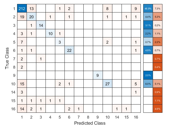
Use the cross-validated ECOC classifier to predict validation-fold labels. You can compute the confusion matrix by using confusionchart. Move and resize the chart by changing the inner position property to ensure that the percentages appear in the row summary.

oofLabel = kfoldPredict(CVMdl,'Options',options);
ConfMat = confusionchart(Y,oofLabel,'RowSummary','total-normalized');
ConfMat.InnerPosition = [0.10 0.12 0.85 0.85];

Reproduce Binned Data

Reproduce binned predictor data by using the BinEdges property of the trained model and the discretize function.

X = Mdl.X; % Predictor data
Xbinned = zeros(size(X));
edges = Mdl.BinEdges;
% Find indices of binned predictors.
idxNumeric = find(~cellfun(@isempty,edges));
if iscolumn(idxNumeric)
    idxNumeric = idxNumeric';
end
for j = idxNumeric 
    x = X(:,j);
    % Convert x to array if x is a table.
    if istable(x)
        x = table2array(x);
    end
    % Group x into bins by using the discretize function.
    xbinned = discretize(x,[-inf; edges{j}; inf]);
    Xbinned(:,j) = xbinned;
end

Xbinned contains the bin indices, ranging from 1 to the number of bins, for numeric predictors. Xbinned values are 0 for categorical predictors. If X contains NaNs, then the corresponding Xbinned values are NaNs.

Optimize ECOC Classifier

Optimize hyperparameters automatically using fitcecoc.

Load the fisheriris data set.

load fisheriris
X = meas;
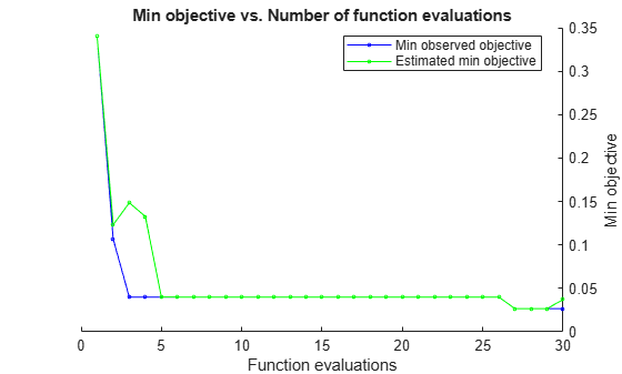
Y = species;

Find hyperparameters that minimize five-fold cross-validation loss by using automatic hyperparameter optimization. For reproducibility, set the random seed and use the 'expected-improvement-plus' acquisition function.

rng default
Mdl = fitcecoc(X,Y,'OptimizeHyperparameters','auto',...
    'HyperparameterOptimizationOptions',struct('AcquisitionFunctionName',...
    'expected-improvement-plus'))

|====================================================================================================================|
| Iter | Eval   | Objective   | Objective   | BestSoFar   | BestSoFar   |       Coding | BoxConstraint|  KernelScale |
|      | result |             | runtime     | (observed)  | (estim.)    |              |              |              |
|====================================================================================================================|
|    1 | Best   |     0.10667 |      1.4394 |     0.10667 |     0.10667 |     onevsone |       5.6939 |       200.36 |
|    2 | Best   |    0.046667 |      3.1683 |    0.046667 |    0.049769 |     onevsone |       94.849 |    0.0032549 |
|    3 | Accept |        0.08 |     0.48573 |    0.046667 |    0.049209 |     onevsall |      0.01378 |     0.076021 |
|    4 | Accept |        0.08 |     0.28785 |    0.046667 |    0.047942 |     onevsall |          889 |       38.798 |
|    5 | Accept |    0.046667 |      1.6891 |    0.046667 |    0.046652 |     onevsone |       2.1285 |    0.0027554 |
|    6 | Best   |        0.04 |     0.24332 |        0.04 |    0.040219 |     onevsone |    0.0020155 |    0.0010001 |
|    7 | Accept |    0.046667 |      1.9448 |        0.04 |    0.043609 |     onevsone |       0.4143 |    0.0010032 |
|    8 | Accept |        0.04 |     0.33928 |        0.04 |    0.039781 |     onevsone |    0.0010403 |    0.0010304 |
|    9 | Accept |    0.046667 |      1.6728 |        0.04 |    0.039758 |     onevsone |       993.63 |     0.064389 |
|   10 | Accept |    0.046667 |     0.52604 |        0.04 |    0.039752 |     onevsone |    0.0010072 |      0.01665 |
|   11 | Accept |        0.04 |     0.79602 |        0.04 |    0.039716 |     onevsone |    0.0010394 |    0.0018643 |
|   12 | Accept |        0.04 |     0.42709 |        0.04 |    0.039928 |     onevsone |     0.001014 |    0.0010761 |
|   13 | Accept |     0.33333 |     0.56692 |        0.04 |    0.039747 |     onevsall |    0.0010661 |       982.42 |
|   14 | Accept |        0.04 |      0.5442 |        0.04 |    0.039738 |     onevsall |       932.91 |       2.9173 |
|   15 | Accept |     0.41333 |      11.994 |        0.04 |    0.039864 |     onevsall |       929.37 |    0.0010004 |
|   16 | Accept |        0.04 |      0.3551 |        0.04 |    0.039887 |     onevsone |       913.75 |       2.7842 |
|   17 | Accept |     0.33333 |     0.45369 |        0.04 |    0.040013 |     onevsall |    0.0011214 |      0.57694 |
|   18 | Accept |        0.04 |     0.36217 |        0.04 |    0.039829 |     onevsall |      0.62669 |     0.096307 |
|   19 | Accept |        0.06 |     0.49719 |        0.04 |    0.039941 |     onevsall |        744.9 |       7.5881 |
|   20 | Accept |     0.10667 |     0.31672 |        0.04 |    0.039948 |     onevsone |    0.0010766 |       2.5209 |
|====================================================================================================================|
| Iter | Eval   | Objective   | Objective   | BestSoFar   | BestSoFar   |       Coding | BoxConstraint|  KernelScale |
|      | result |             | runtime     | (observed)  | (estim.)    |              |              |              |
|====================================================================================================================|
|   21 | Accept |     0.14667 |      7.7979 |        0.04 |    0.040006 |     onevsall |       979.04 |      0.15295 |
|   22 | Accept |    0.046667 |      3.6765 |        0.04 |    0.040008 |     onevsall |     0.023947 |    0.0032873 |
|   23 | Accept |    0.046667 |     0.46689 |        0.04 |    0.040005 |     onevsone |       6.3496 |      0.46716 |
|   24 | Accept |    0.046667 |     0.64157 |        0.04 |    0.040003 |     onevsall |     0.091577 |     0.019408 |
|   25 | Accept |    0.046667 |      3.2627 |        0.04 |    0.040002 |     onevsall |     0.001022 |    0.0010928 |
|   26 | Accept |    0.046667 |      0.3478 |        0.04 |    0.040001 |     onevsall |       29.705 |       1.0323 |
|   27 | Accept |     0.10667 |     0.26668 |        0.04 |    0.040001 |     onevsone |       959.24 |       989.48 |
|   28 | Accept |        0.04 |     0.51226 |        0.04 |    0.040003 |     onevsone |      0.16662 |      0.04099 |
|   29 | Accept |     0.10667 |     0.25919 |        0.04 |    0.040004 |     onevsone |    0.0010206 |       959.92 |
|   30 | Accept |        0.04 |     0.39581 |        0.04 |    0.040004 |     onevsall |    0.0028825 |    0.0053013 |

__________________________________________________________
Optimization completed.
MaxObjectiveEvaluations of 30 reached.
Total function evaluations: 30
Total elapsed time: 61.7358 seconds
Total objective function evaluation time: 45.7374

Best observed feasible point:
     Coding     BoxConstraint    KernelScale
    ________    _____________    ___________

    onevsone      0.0020155       0.0010001 

Observed objective function value = 0.04
Estimated objective function value = 0.039977
Function evaluation time = 0.24332

Best estimated feasible point (according to models):
     Coding     BoxConstraint    KernelScale
    ________    _____________    ___________

    onevsone      0.001014        0.0010761 

Estimated objective function value = 0.040004
Estimated function evaluation time = 0.44278

Mdl = 
  ClassificationECOC
                         ResponseName: 'Y'
                CategoricalPredictors: []
                           ClassNames: {'setosa'  'versicolor'  'virginica'}
                       ScoreTransform: 'none'
                       BinaryLearners: {3x1 cell}
                           CodingName: 'onevsone'
    HyperparameterOptimizationResults: [1x1 BayesianOptimization]


  Properties, Methods

Train Multiclass ECOC Model with SVMs and Tall Arrays

Create two multiclass ECOC models trained on tall data. Use linear binary learners for one of the models and kernel binary learners for the other. Compare the resubstitution classification error of the two models.

In general, you can perform multiclass classification of tall data by using fitcecoc with linear or kernel binary learners. When you use fitcecoc to train a model on tall arrays, you cannot use SVM binary learners directly. However, you can use either linear or kernel binary classification models that use SVMs.

When you perform calculations on tall arrays, MATLAB® uses either a parallel pool (default if you have Parallel Computing Toolbox™) or the local MATLAB session. If you want to run the example using the local MATLAB session when you have Parallel Computing Toolbox, you can change the global execution environment by using the mapreducer function.

Create a datastore that references the folder containing Fisher's iris data set. Specify 'NA' values as missing data so that datastore replaces them with NaN values. Create tall versions of the predictor and response data.

ds = datastore('fisheriris.csv','TreatAsMissing','NA');
t = tall(ds);

Starting parallel pool (parpool) using the 'local' profile ...
Connected to the parallel pool (number of workers: 6).

X = [t.SepalLength t.SepalWidth t.PetalLength t.PetalWidth];
Y = t.Species;

Standardize the predictor data.

Z = zscore(X);

Train a multiclass ECOC model that uses tall data and linear binary learners. By default, when you pass tall arrays to fitcecoc, the software trains linear binary learners that use SVMs. Because the response data contains only three unique classes, change the coding scheme from one-versus-all (which is the default when you use tall data) to one-versus-one (which is the default when you use in-memory data).

For reproducibility, set the seeds of the random number generators using rng and tallrng. The results can vary depending on the number of workers and the execution environment for the tall arrays. For details, see Control Where Your Code Runs.

rng('default') 
tallrng('default')
mdlLinear = fitcecoc(Z,Y,'Coding','onevsone')

Training binary learner 1 (Linear) out of 3.
Training binary learner 2 (Linear) out of 3.
Training binary learner 3 (Linear) out of 3.

mdlLinear = 
  CompactClassificationECOC
      ResponseName: 'Y'
        ClassNames: {'setosa'  'versicolor'  'virginica'}
    ScoreTransform: 'none'
    BinaryLearners: {3×1 cell}
      CodingMatrix: [3×3 double]


  Properties, Methods

mdlLinear is a CompactClassificationECOC model composed of three binary learners.

Train a multiclass ECOC model that uses tall data and kernel binary learners. First, create a templateKernel object to specify the properties of the kernel binary learners; in particular, increase the number of expansion dimensions to $$2^{16}$$.

tKernel = templateKernel('NumExpansionDimensions',2^16)

tKernel = 
Fit template for classification Kernel.

             BetaTolerance: []
                 BlockSize: []
             BoxConstraint: []
                   Epsilon: []
    NumExpansionDimensions: 65536
         GradientTolerance: []
        HessianHistorySize: []
            IterationLimit: []
               KernelScale: []
                    Lambda: []
                   Learner: 'svm'
              LossFunction: []
                    Stream: []
            VerbosityLevel: []
                   Version: 1
                    Method: 'Kernel'
                      Type: 'classification'

By default, the kernel binary learners use SVMs.

Pass the templateKernel object to fitcecoc and change the coding scheme to one-versus-one.

mdlKernel = fitcecoc(Z,Y,'Learners',tKernel,'Coding','onevsone')

Training binary learner 1 (Kernel) out of 3.
Training binary learner 2 (Kernel) out of 3.
Training binary learner 3 (Kernel) out of 3.

mdlKernel = 
  CompactClassificationECOC
      ResponseName: 'Y'
        ClassNames: {'setosa'  'versicolor'  'virginica'}
    ScoreTransform: 'none'
    BinaryLearners: {3×1 cell}
      CodingMatrix: [3×3 double]


  Properties, Methods

mdlKernel is also a CompactClassificationECOC model composed of three binary learners.

Compare the resubstitution classification error of the two models.

errorLinear = gather(loss(mdlLinear,Z,Y))

Evaluating tall expression using the Parallel Pool 'local':
- Pass 1 of 1: Completed in 1.4 sec
Evaluation completed in 1.6 sec

errorLinear = 0.0333

errorKernel = gather(loss(mdlKernel,Z,Y))

Evaluating tall expression using the Parallel Pool 'local':
- Pass 1 of 1: Completed in 15 sec
Evaluation completed in 16 sec

errorKernel = 0.0067

mdlKernel misclassifies a smaller percentage of the training data than mdlLinear.

Input Arguments

Tbl — Sample data

table

Sample data, specified as a table. Each row of Tbl corresponds to one observation, and each column corresponds to one predictor. Optionally, Tbl can contain one additional column for the response variable. Multicolumn variables and cell arrays other than cell arrays of character vectors are not accepted.

If Tbl contains the response variable, and you want to use all remaining variables in Tbl as predictors, then specify the response variable using ResponseVarName.

If Tbl contains the response variable, and you want to use only a subset of the remaining variables in Tbl as predictors, specify a formula using formula.

If Tbl does not contain the response variable, specify a response variable using Y. The length of response variable and the number of Tbl rows must be equal.

Data Types: table

ResponseVarName — Response variable name

name of variable in Tbl

Response variable name, specified as the name of a variable in Tbl.

You must specify ResponseVarName as a character vector or string scalar. For example, if the response variable Y is stored as Tbl.Y, then specify it as "Y". Otherwise, the software treats all columns of Tbl, including Y, as predictors when training the model.

The response variable must be a categorical, character, or string array; a logical or numeric vector; or a cell array of character vectors. If Y is a character array, then each element of the response variable must correspond to one row of the array.

A good practice is to specify the order of the classes by using the ClassNames name-value argument.

Data Types: char | string

formula — Explanatory model of response variable and subset of predictor variables

character vector | string scalar

Explanatory model of the response variable and a subset of the predictor variables, specified as a character vector or string scalar in the form "Y~x1+x2+x3". In this form, Y represents the response variable, and x1, x2, and x3 represent the predictor variables.

To specify a subset of variables in Tbl as predictors for training the model, use a formula. If you specify a formula, then the software does not use any variables in Tbl that do not appear in formula.

The variable names in the formula must be both variable names in Tbl (Tbl.Properties.VariableNames) and valid MATLAB^® identifiers. You can verify the variable names in Tbl by using the isvarname function. If the variable names are not valid, then you can convert them by using the matlab.lang.makeValidName function.

Data Types: char | string

Y — Class labels

categorical array | character array | string array | logical vector | numeric vector | cell array of character vectors

Class labels to which the ECOC model is trained, specified as a categorical, character, or string array, logical or numeric vector, or cell array of character vectors.

If Y is a character array, then each element must correspond to one row of the array.

The length of Y and the number of rows of Tbl or X must be equal.

It is good practice to specify the class order using the ClassNames name-value pair argument.

Data Types: categorical | char | string | logical | single | double | cell

X — Predictor data

full matrix | sparse matrix

Predictor data, specified as a full or sparse matrix.

The length of Y and the number of observations in X must be equal.

To specify the names of the predictors in the order of their appearance in X, use the PredictorNames name-value pair argument.

Note

• For linear classification learners, if you orient X so that observations correspond to columns and specify 'ObservationsIn','columns', then you can experience a significant reduction in optimization-execution time.

• For all other learners, orient X so that observations correspond to rows.

• fitcecoc supports sparse matrices for training linear classification models only.

Data Types: double | single

Note

The software treats NaN, empty character vector (''), empty string (""), <missing>, and <undefined> elements as missing data. The software removes rows of X corresponding to missing values in Y. However, the treatment of missing values in X varies among binary learners. For details, see the training functions for your binary learners: fitcdiscr, fitckernel, fitcknn, fitclinear, fitcnb, fitcsvm, fitctree, or fitcensemble. Removing observations decreases the effective training or cross-validation sample size.

Name-Value Arguments

Specify optional comma-separated pairs of Name,Value arguments. Name is the argument name and Value is the corresponding value. Name must appear inside quotes. You can specify several name and value pair arguments in any order as Name1,Value1,...,NameN,ValueN.

Example: 'Learners','tree','Coding','onevsone','CrossVal','on' specifies to use decision trees for all binary learners, a one-versus-one coding design, and to implement 10-fold cross-validation.

Note

You cannot use any cross-validation name-value argument together with the 'OptimizeHyperparameters' name-value argument. You can modify the cross-validation for 'OptimizeHyperparameters' only by using the 'HyperparameterOptimizationOptions' name-value argument.

ECOC Classifier Options

Coding — Coding design

'onevsone' (default) | 'allpairs' | 'binarycomplete' | 'denserandom' | 'onevsall' | 'ordinal' | 'sparserandom' | 'ternarycomplete' | numeric matrix

Coding design name, specified as the comma-separated pair consisting of 'Coding' and a numeric matrix or a value in this table.

Value	Number of Binary Learners	Description
'allpairs' and 'onevsone'	K(K – 1)/2	For each binary learner, one class is positive, another is negative, and the software ignores the rest. This design exhausts all combinations of class pair assignments.
'binarycomplete'	$$2^{(K-1)}-1$$	This design partitions the classes into all binary combinations, and does not ignore any classes. For each binary learner, all class assignments are -1 and 1 with at least one positive and negative class in the assignment.
'denserandom'	Random, but approximately 10 log2K	For each binary learner, the software randomly assigns classes into positive or negative classes, with at least one of each type. For more details, see Random Coding Design Matrices.
'onevsall'	K	For each binary learner, one class is positive and the rest are negative. This design exhausts all combinations of positive class assignments.
'ordinal'	K – 1	For the first binary learner, the first class is negative, and the rest positive. For the second binary learner, the first two classes are negative, the rest positive, and so on.
'sparserandom'	Random, but approximately 15 log2K	For each binary learner, the software randomly assigns classes as positive or negative with probability 0.25 for each, and ignores classes with probability 0.5. For more details, see Random Coding Design Matrices.
'ternarycomplete'	$$\left(3^K-2^{(K+1)}+1\right)/2$$	This design partitions the classes into all ternary combinations. All class assignments are 0, -1, and 1 with at least one positive and one negative class in the assignment.

You can also specify a coding design using a custom coding matrix. The custom coding matrix is a K-by-L matrix. Each row corresponds to a class and each column corresponds to a binary learner. The class order (rows) corresponds to the order in ClassNames. Compose the matrix by following these guidelines:

• Every element of the custom coding matrix must be -1, 0, or 1, and the value must correspond to a dichotomous class assignment. This table describes the meaning of Coding(i,j), that is, the class that learner j assigns to observations in class i.

  Value	Dichotomous Class Assignment
  –1	Learner j assigns observations in class i to a negative class.
  0	Before training, learner j removes observations in class i from the data set.
  1	Learner j assigns observations in class i to a positive class.

• Every column must contain at least one -1 or 1.

• For all column indices i,j such that i ≠ j, Coding(:,i) cannot equal Coding(:,j) and Coding(:,i) cannot equal -Coding(:,j).

• All rows of the custom coding matrix must be different.

For more details on the form of custom coding design matrices, see Custom Coding Design Matrices.

Example: 'Coding','ternarycomplete'

Data Types: char | string | double | single | int16 | int32 | int64 | int8

FitPosterior — Flag indicating whether to transform scores to posterior probabilities

false or 0 (default) | true or 1

Flag indicating whether to transform scores to posterior probabilities, specified as the comma-separated pair consisting of 'FitPosterior' and a true (1) or false (0).

If FitPosterior is true, then the software transforms binary-learner classification scores to posterior probabilities. You can obtain posterior probabilities by using kfoldPredict, predict, or resubPredict.

fitcecoc does not support fitting posterior probabilities if:

• The ensemble method is AdaBoostM2, LPBoost, RUSBoost, RobustBoost, or TotalBoost.

• The binary learners (Learners) are linear or kernel classification models that implement SVM. To obtain posterior probabilities for linear or kernel classification models, implement logistic regression instead.

Example: 'FitPosterior',true

Data Types: logical

Learners — Binary learner templates

'svm' (default) | 'discriminant' | 'kernel' | 'knn' | 'linear' | 'naivebayes' | 'tree' | template object | cell vector of template objects

Binary learner templates, specified as the comma-separated pair consisting of 'Learners' and a character vector, string scalar, template object, or cell vector of template objects. Specifically, you can specify binary classifiers such as SVM, and the ensembles that use GentleBoost, LogitBoost, and RobustBoost, to solve multiclass problems. However, fitcecoc also supports multiclass models as binary classifiers.

• If Learners is a character vector or string scalar, then the software trains each binary learner using the default values of the specified algorithm. This table summarizes the available algorithms.

  Value	Description
  'discriminant'	Discriminant analysis. For default options, see templateDiscriminant.
  'kernel'	Kernel classification model. For default options, see templateKernel.
  'knn'	k-nearest neighbors. For default options, see templateKNN.
  'linear'	Linear classification model. For default options, see templateLinear.
  'naivebayes'	Naive Bayes. For default options, see templateNaiveBayes.
  'svm'	SVM. For default options, see templateSVM.
  'tree'	Classification trees. For default options, see templateTree.

• If Learners is a template object, then each binary learner trains according to the stored options. You can create a template object using:

  • templateDiscriminant, for discriminant analysis.

  • templateEnsemble, for ensemble learning. You must at least specify the learning method (Method), the number of learners (NLearn), and the type of learner (Learners). You cannot use the AdaBoostM2 ensemble method for binary learning.

  • templateKernel, for kernel classification.

  • templateKNN, for k-nearest neighbors.

  • templateLinear, for linear classification.

  • templateNaiveBayes, for naive Bayes.

  • templateSVM, for SVM.

  • templateTree, for classification trees.

• If Learners is a cell vector of template objects, then:

  • Cell j corresponds to binary learner j (in other words, column j of the coding design matrix), and the cell vector must have length L. L is the number of columns in the coding design matrix. For details, see Coding.

  • To use one of the built-in loss functions for prediction, then all binary learners must return a score in the same range. For example, you cannot include default SVM binary learners with default naive Bayes binary learners. The former returns a score in the range (-∞,∞), and the latter returns a posterior probability as a score. Otherwise, you must provide a custom loss as a function handle to functions such as predict and loss.

  • You cannot specify linear classification model learner templates with any other template.

  • Similarly, you cannot specify kernel classification model learner templates with any other template.

By default, the software trains learners using default SVM templates.

Example: 'Learners','tree'

NumBins — Number of bins for numeric predictors

[](empty) (default) | positive integer scalar

Number of bins for numeric predictors, specified as the comma-separated pair consisting of 'NumBins' and a positive integer scalar. This argument is valid only when fitcecoc uses a tree learner, that is, 'Learners' is either 'tree' or a template object created by using templateTree, or a template object created by using templateEnsemble with tree weak learners.

• If the 'NumBins' value is empty (default), then fitcecoc does not bin any predictors.

• If you specify the 'NumBins' value as a positive integer scalar (numBins), then fitcecoc bins every numeric predictor into at most numBins equiprobable bins, and then grows trees on the bin indices instead of the original data.

  • The number of bins can be less than numBins if a predictor has fewer than numBins unique values.

  • fitcecoc does not bin categorical predictors.

When you use a large training data set, this binning option speeds up training but might cause a potential decrease in accuracy. You can try 'NumBins',50 first, and then change the value depending on the accuracy and training speed.

A trained model stores the bin edges in the BinEdges property.

Example: 'NumBins',50

Data Types: single | double

NumConcurrent — Number of binary learners concurrently trained

1 (default) | positive integer scalar

Number of binary learners concurrently trained, specified as the comma-separated pair consisting of 'NumConcurrent' and a positive integer scalar. The default value is 1, which means fitcecoc trains the binary learners sequentially.

Note

This option applies only when you use fitcecoc on tall arrays. See Tall Arrays for more information.

Data Types: single | double

ObservationsIn — Predictor data observation dimension

'rows' (default) | 'columns'

Predictor data observation dimension, specified as the comma-separated pair consisting of 'ObservationsIn' and 'columns' or 'rows'.

Note

• For linear classification learners, if you orient X so that observations correspond to columns and specify 'ObservationsIn','columns', then you can experience a significant reduction in optimization-execution time.

• For all other learners, orient X so that observations correspond to rows.

Example: 'ObservationsIn','columns'

Verbose — Verbosity level

0 (default) | 1 | 2

Verbosity level, specified as the comma-separated pair consisting of 'Verbose' and 0, 1, or 2. Verbose controls the amount of diagnostic information per binary learner that the software displays in the Command Window.

This table summarizes the available verbosity level options.

Value	Description
0	The software does not display diagnostic information.
1	The software displays diagnostic messages every time it trains a new binary learner.
2	The software displays extra diagnostic messages every time it trains a new binary learner.

Each binary learner has its own verbosity level that is independent of this name-value pair argument. To change the verbosity level of a binary learner, create a template object and specify the 'Verbose' name-value pair argument. Then, pass the template object to fitcecoc by using the 'Learners' name-value pair argument.

Example: 'Verbose',1

Data Types: double | single

Cross-Validation Options

CrossVal — Flag to train cross-validated classifier

'off' (default) | 'on'

Flag to train a cross-validated classifier, specified as the comma-separated pair consisting of 'Crossval' and 'on' or 'off'.

If you specify 'on', then the software trains a cross-validated classifier with 10 folds.

You can override this cross-validation setting using one of the CVPartition, Holdout, KFold, or Leaveout name-value pair arguments. You can only use one cross-validation name-value pair argument at a time to create a cross-validated model.

Alternatively, cross-validate later by passing Mdl to crossval.

Example: 'Crossval','on'

CVPartition — Cross-validation partition

[] (default) | cvpartition partition object

Cross-validation partition, specified as a cvpartition partition object created by cvpartition. The partition object specifies the type of cross-validation and the indexing for the training and validation sets.

To create a cross-validated model, you can specify only one of these four name-value arguments: CVPartition, Holdout, KFold, or Leaveout.

Example: Suppose you create a random partition for 5-fold cross-validation on 500 observations by using cvp = cvpartition(500,'KFold',5). Then, you can specify the cross-validated model by using 'CVPartition',cvp.

Holdout — Fraction of data for holdout validation

scalar value in the range (0,1)

Fraction of the data used for holdout validation, specified as a scalar value in the range (0,1). If you specify 'Holdout',p, then the software completes these steps:

1. Randomly select and reserve p*100% of the data as validation data, and train the model using the rest of the data.

2. Store the compact, trained model in the Trained property of the cross-validated model.

To create a cross-validated model, you can specify only one of these four name-value arguments: CVPartition, Holdout, KFold, or Leaveout.

Example: 'Holdout',0.1

Data Types: double | single

KFold — Number of folds

10 (default) | positive integer value greater than 1

Number of folds to use in a cross-validated model, specified as a positive integer value greater than 1. If you specify 'KFold',k, then the software completes these steps:

1. Randomly partition the data into k sets.

2. For each set, reserve the set as validation data, and train the model using the other k – 1 sets.

3. Store the k compact, trained models in a k-by-1 cell vector in the Trained property of the cross-validated model.

To create a cross-validated model, you can specify only one of these four name-value arguments: CVPartition, Holdout, KFold, or Leaveout.

Example: 'KFold',5

Data Types: single | double

Leaveout — Leave-one-out cross-validation flag

'off' (default) | 'on'

Leave-one-out cross-validation flag, specified as the comma-separated pair consisting of 'Leaveout' and 'on' or 'off'. If you specify 'Leaveout','on', then, for each of the n observations, where n is size(Mdl.X,1), the software:

1. Reserves the observation as validation data, and trains the model using the other n – 1 observations

2. Stores the n compact, trained models in the cells of a n-by-1 cell vector in the Trained property of the cross-validated model.

To create a cross-validated model, you can use one of these four options only: CVPartition, Holdout, KFold, or Leaveout.

Note

Leave-one-out is not recommended for cross-validating ECOC models composed of linear or kernel classification model learners.

Example: 'Leaveout','on'

Other Classification Options

CategoricalPredictors — Categorical predictors list

vector of positive integers | logical vector | character matrix | string array | cell array of character vectors | 'all'

Categorical predictors list, specified as one of the values in this table.

Value	Description
Vector of positive integers	Each entry in the vector is an index value indicating that the corresponding predictor is categorical. The index values are between 1 and p, where p is the number of predictors used to train the model. If fitcecoc uses a subset of input variables as predictors, then the function indexes the predictors using only the subset. The CategoricalPredictors values do not count the response variable, observation weight variable, or any other variables that the function does not use.
Logical vector	A true entry means that the corresponding predictor is categorical. The length of the vector is p.
Character matrix	Each row of the matrix is the name of a predictor variable. The names must match the entries in PredictorNames. Pad the names with extra blanks so each row of the character matrix has the same length.
String array or cell array of character vectors	Each element in the array is the name of a predictor variable. The names must match the entries in PredictorNames.
"all"	All predictors are categorical.

Specification of 'CategoricalPredictors' is appropriate if:

• At least one predictor is categorical and all binary learners are classification trees, naive Bayes learners, SVMs, linear learners, kernel learners, or ensembles of classification trees.

• All predictors are categorical and at least one binary learner is kNN.

If you specify 'CategoricalPredictors' for any other learner, then the software warns that it cannot train that binary learner. For example, the software cannot train discriminant analysis classifiers using categorical predictors.

Each learner identifies and treats categorical predictors in the same way as the fitting function corresponding to the learner. See 'CategoricalPredictors' of fitckernel for kernel learners, 'CategoricalPredictors' of fitcknn for k-nearest learners, 'CategoricalPredictors' of fitclinear for linear learners, 'CategoricalPredictors' of fitcnb for naive Bayes learners, 'CategoricalPredictors' of fitcsvm for SVM learners, and 'CategoricalPredictors' of fitctree for tree learners.

Example: 'CategoricalPredictors','all'

Data Types: single | double | logical | char | string | cell

ClassNames — Names of classes to use for training

categorical array | character array | string array | logical vector | numeric vector | cell array of character vectors

Names of classes to use for training, specified as a categorical, character, or string array; a logical or numeric vector; or a cell array of character vectors. ClassNames must have the same data type as the response variable in Tbl or Y.

If ClassNames is a character array, then each element must correspond to one row of the array.

Use ClassNames to:

• Specify the order of the classes during training.

• Specify the order of any input or output argument dimension that corresponds to the class order. For example, use ClassNames to specify the order of the dimensions of Cost or the column order of classification scores returned by predict.

• Select a subset of classes for training. For example, suppose that the set of all distinct class names in Y is ["a","b","c"]. To train the model using observations from classes "a" and "c" only, specify "ClassNames",["a","c"].

The default value for ClassNames is the set of all distinct class names in the response variable in Tbl or Y.

Example: "ClassNames",["b","g"]

Data Types: categorical | char | string | logical | single | double | cell

Cost — Misclassification cost

square matrix | structure array

Misclassification cost, specified as the comma-separated pair consisting of 'Cost' and a square matrix or structure. If you specify:

• The square matrix Cost, then Cost(i,j) is the cost of classifying a point into class j if its true class is i. That is, the rows correspond to the true class and the columns correspond to the predicted class. To specify the class order for the corresponding rows and columns of Cost, additionally specify the ClassNames name-value pair argument.

• The structure S, then it must have two fields:

  • S.ClassNames, which contains the class names as a variable of the same data type as Y

  • S.ClassificationCosts, which contains the cost matrix with rows and columns ordered as in S.ClassNames

The default is ones(K) - eye(K), where K is the number of distinct classes.

Example: 'Cost',[0 1 2 ; 1 0 2; 2 2 0]

Data Types: double | single | struct

Options — Parallel computing options

[] (default) | structure array returned by statset

Parallel computing options, specified as the comma-separated pair consisting of 'Options' and a structure array returned by statset. These options require Parallel Computing Toolbox™. fitcecoc uses 'Streams', 'UseParallel', and 'UseSubtreams' fields.

This table summarizes the available options.

Option	Description
'Streams'	A RandStream object or cell array of such objects. If you do not specify Streams, the software uses the default stream or streams. If you specify Streams, use a single object except when the following are true: You have an open parallel pool. UseParallel is true. UseSubstreams is false. In that case, use a cell array of the same size as the parallel pool. If a parallel pool is not open, then the software tries to open one (depending on your preferences), and Streams must supply a single random number stream.
'UseParallel'	If you have Parallel Computing Toolbox, then you can invoke a pool of workers by setting 'UseParallel',true. The fitcecoc function sends each binary learner to a worker in the pool. When you use decision trees for binary learners, fitcecoc parallelizes training using Intel® Threading Building Blocks (TBB) for dual-core systems and above. Therefore, specifying the 'UseParallel' option is not helpful on a single computer. Use this option on a cluster. For details on Intel TBB, see https://software.intel.com/content/www/us/en/develop/tools/oneapi/components/onetbb.html.
'UseSubstreams'	Set to true to compute in parallel using the stream specified by 'Streams'. Default is false. For example, set Streams to a type allowing substreams, such as'mlfg6331_64' or 'mrg32k3a'.

A best practice to ensure more predictable results is to use parpool (Parallel Computing Toolbox) and explicitly create a parallel pool before you invoke parallel computing using fitcecoc.

Example: 'Options',statset('UseParallel',true)

Data Types: struct

PredictorNames — Predictor variable names

string array of unique names | cell array of unique character vectors

Predictor variable names, specified as a string array of unique names or cell array of unique character vectors. The functionality of PredictorNames depends on the way you supply the training data.

• If you supply X and Y, then you can use PredictorNames to assign names to the predictor variables in X.

  • The order of the names in PredictorNames must correspond to the column order of X. That is, PredictorNames{1} is the name of X(:,1), PredictorNames{2} is the name of X(:,2), and so on. Also, size(X,2) and numel(PredictorNames) must be equal.

  • By default, PredictorNames is {'x1','x2',...}.

• If you supply Tbl, then you can use PredictorNames to choose which predictor variables to use in training. That is, fitcecoc uses only the predictor variables in PredictorNames and the response variable during training.

  • PredictorNames must be a subset of Tbl.Properties.VariableNames and cannot include the name of the response variable.

  • By default, PredictorNames contains the names of all predictor variables.

  • A good practice is to specify the predictors for training using either PredictorNames or formula, but not both.

Example: "PredictorNames",["SepalLength","SepalWidth","PetalLength","PetalWidth"]

Data Types: string | cell

Prior — Prior probabilities

'empirical' (default) | 'uniform' | numeric vector | structure array

Prior probabilities for each class, specified as the comma-separated pair consisting of 'Prior' and a value in this table.

Value	Description
'empirical'	The class prior probabilities are the class relative frequencies in Y.
'uniform'	All class prior probabilities are equal to 1/K, where K is the number of classes.
numeric vector	Each element is a class prior probability. Order the elements according to Mdl.ClassNames or specify the order using the ClassNames name-value pair argument. The software normalizes the elements such that they sum to 1.
structure	A structure S with two fields: S.ClassNames contains the class names as a variable of the same type as Y. S.ClassProbs contains a vector of corresponding prior probabilities. The software normalizes the elements such that they sum to 1.

For more details on how the software incorporates class prior probabilities, see Prior Probabilities and Cost.

Example: struct('ClassNames',{{'setosa','versicolor','virginica'}},'ClassProbs',1:3)

Data Types: single | double | char | string | struct

ResponseName — Response variable name

"Y" (default) | character vector | string scalar

Response variable name, specified as a character vector or string scalar.

• If you supply Y, then you can use ResponseName to specify a name for the response variable.

• If you supply ResponseVarName or formula, then you cannot use ResponseName.

Example: "ResponseName","response"

Data Types: char | string

ScoreTransform — Score transformation

"none" (default) | "doublelogit" | "invlogit" | "ismax" | "logit" | function handle | ...

Score transformation, specified as a character vector, string scalar, or function handle.

This table summarizes the available character vectors and string scalars.

Value	Description
"doublelogit"	1/(1 + e–2x)
"invlogit"	log(x / (1 – x))
"ismax"	Sets the score for the class with the largest score to 1, and sets the scores for all other classes to 0
"logit"	1/(1 + e–x)
"none" or "identity"	x (no transformation)
"sign"	–1 for x < 0 0 for x = 0 1 for x > 0
"symmetric"	2x – 1
"symmetricismax"	Sets the score for the class with the largest score to 1, and sets the scores for all other classes to –1
"symmetriclogit"	2/(1 + e–x) – 1

For a MATLAB function or a function you define, use its function handle for the score transform. The function handle must accept a matrix (the original scores) and return a matrix of the same size (the transformed scores).

Example: "ScoreTransform","logit"

Data Types: char | string | function_handle

Weights — Observation weights

numeric vector of positive values | name of variable in Tbl

Observation weights, specified as the comma-separated pair consisting of 'Weights' and a numeric vector of positive values or name of a variable in Tbl. The software weighs the observations in each row of X or Tbl with the corresponding value in Weights. The size of Weights must equal the number of rows of X or Tbl.

If you specify the input data as a table Tbl, then Weights can be the name of a variable in Tbl that contains a numeric vector. In this case, you must specify Weights as a character vector or string scalar. For example, if the weights vector W is stored as Tbl.W, then specify it as 'W'. Otherwise, the software treats all columns of Tbl, including W, as predictors or the response when training the model.

The software normalizes Weights to sum up to the value of the prior probability in the respective class.

By default, Weights is ones(n,1), where n is the number of observations in X or Tbl.

Data Types: double | single | char | string

Hyperparameter Optimization

OptimizeHyperparameters — Parameters to optimize

'none' (default) | 'auto' | 'all' | string array or cell array of eligible parameter names | vector of optimizableVariable objects

Parameters to optimize, specified as the comma-separated pair consisting of 'OptimizeHyperparameters' and one of the following:

• 'none' — Do not optimize.

• 'auto' — Use {'Coding'} along with the default parameters for the specified Learners:

  • Learners = 'svm' (default) — {'BoxConstraint','KernelScale'}

  • Learners = 'discriminant' — {'Delta','Gamma'}

  • Learners = 'kernel' — {'KernelScale','Lambda'}

  • Learners = 'knn' — {'Distance','NumNeighbors'}

  • Learners = 'linear' — {'Lambda','Learner'}

  • Learners = 'naivebayes' — {'DistributionNames','Width'}

  • Learners = 'tree' — {'MinLeafSize'}

• 'all' — Optimize all eligible parameters.

• String array or cell array of eligible parameter names

• Vector of optimizableVariable objects, typically the output of hyperparameters

The optimization attempts to minimize the cross-validation loss (error) for fitcecoc by varying the parameters. For information about cross-validation loss in a different context, see Classification Loss. To control the cross-validation type and other aspects of the optimization, use the HyperparameterOptimizationOptions name-value pair.

Note

The values of 'OptimizeHyperparameters' override any values you specify using other name-value arguments. For example, setting 'OptimizeHyperparameters' to 'auto' causes fitcecoc to optimize hyperparameters corresponding to the 'auto' option and to ignore any specified values for the hyperparameters.

The eligible parameters for fitcecoc are:

• Coding — fitcecoc searches among 'onevsall' and 'onevsone'.

• The eligible hyperparameters for the chosen Learners, as specified in this table.

  Learners	Eligible Hyperparameters (Bold = Default)	Default Range
  'discriminant'	Delta	Log-scaled in the range [1e-6,1e3]
  	DiscrimType	'linear', 'quadratic', 'diagLinear', 'diagQuadratic', 'pseudoLinear', and 'pseudoQuadratic'
  	Gamma	Real values in [0,1]
  'kernel'	Lambda	Positive values log-scaled in the range [1e-3/NumObservations,1e3/NumObservations]
  	KernelScale	Positive values log-scaled in the range [1e-3,1e3]
  	Learner	'svm' and 'logistic'
  	NumExpansionDimensions	Integers log-scaled in the range [100,10000]
  'knn'	Distance	'cityblock', 'chebychev', 'correlation', 'cosine', 'euclidean', 'hamming', 'jaccard', 'mahalanobis', 'minkowski', 'seuclidean', and 'spearman'
  	DistanceWeight	'equal', 'inverse', and 'squaredinverse'
  	Exponent	Positive values in [0.5,3]
  	NumNeighbors	Positive integer values log-scaled in the range [1, max(2,round(NumObservations/2))]
  	Standardize	'true' and 'false'
  'linear'	Lambda	Positive values log-scaled in the range [1e-5/NumObservations,1e5/NumObservations]
  	Learner	'svm' and 'logistic'
  	Regularization	'ridge' and 'lasso'
  'naivebayes'	DistributionNames	'normal' and 'kernel'
  	Width	Positive values log-scaled in the range [MinPredictorDiff/4,max(MaxPredictorRange,MinPredictorDiff)]
  	Kernel	'normal', 'box', 'epanechnikov', and 'triangle'
  'svm'	BoxConstraint	Positive values log-scaled in the range [1e-3,1e3]
  	KernelScale	Positive values log-scaled in the range [1e-3,1e3]
  	KernelFunction	'gaussian', 'linear', and 'polynomial'
  	PolynomialOrder	Integers in the range [2,4]
  	Standardize	'true' and 'false'
  'tree'	MaxNumSplits	Integers log-scaled in the range [1,max(2,NumObservations-1)]
  	MinLeafSize	Integers log-scaled in the range [1,max(2,floor(NumObservations/2))]
  	NumVariablesToSample	Integers in the range [1,max(2,NumPredictors)]
  	SplitCriterion	'gdi', 'deviance', and 'twoing'

  Alternatively, use hyperparameters with your chosen Learners, such as

  load fisheriris % hyperparameters requires data and learner
  params = hyperparameters('fitcecoc',meas,species,'svm');

  To see the eligible and default hyperparameters, examine params.

Set nondefault parameters by passing a vector of optimizableVariable objects that have nondefault values. For example,

load fisheriris
params = hyperparameters('fitcecoc',meas,species,'svm');
params(2).Range = [1e-4,1e6];

Pass params as the value of OptimizeHyperparameters.

By default, the iterative display appears at the command line, and plots appear according to the number of hyperparameters in the optimization. For the optimization and plots, the objective function is the misclassification rate. To control the iterative display, set the Verbose field of the 'HyperparameterOptimizationOptions' name-value argument. To control the plots, set the ShowPlots field of the 'HyperparameterOptimizationOptions' name-value argument.

For an example, see Optimize ECOC Classifier.

Example: 'auto'

HyperparameterOptimizationOptions — Options for optimization

structure

Options for optimization, specified as a structure. This argument modifies the effect of the OptimizeHyperparameters name-value argument. All fields in the structure are optional.

Field Name	Values	Default
Optimizer	'bayesopt' — Use Bayesian optimization. Internally, this setting calls bayesopt. 'gridsearch' — Use grid search with NumGridDivisions values per dimension. 'randomsearch' — Search at random among MaxObjectiveEvaluations points. 'gridsearch' searches in a random order, using uniform sampling without replacement from the grid. After optimization, you can get a table in grid order by using the command sortrows(Mdl.HyperparameterOptimizationResults).	'bayesopt'
AcquisitionFunctionName	'expected-improvement-per-second-plus' 'expected-improvement' 'expected-improvement-plus' 'expected-improvement-per-second' 'lower-confidence-bound' 'probability-of-improvement' Acquisition functions whose names include per-second do not yield reproducible results because the optimization depends on the runtime of the objective function. Acquisition functions whose names include plus modify their behavior when they are overexploiting an area. For more details, see Acquisition Function Types.	'expected-improvement-per-second-plus'
MaxObjectiveEvaluations	Maximum number of objective function evaluations.	30 for 'bayesopt' and 'randomsearch', and the entire grid for 'gridsearch'
MaxTime	Time limit, specified as a positive real scalar. The time limit is in seconds, as measured by tic and toc. The run time can exceed MaxTime because MaxTime does not interrupt function evaluations.	Inf
NumGridDivisions	For 'gridsearch', the number of values in each dimension. The value can be a vector of positive integers giving the number of values for each dimension, or a scalar that applies to all dimensions. This field is ignored for categorical variables.	10
ShowPlots	Logical value indicating whether to show plots. If true, this field plots the best observed objective function value against the iteration number. If you use Bayesian optimization (Optimizer is 'bayesopt'), then this field also plots the best estimated objective function value. The best observed objective function values and best estimated objective function values correspond to the values in the BestSoFar (observed) and BestSoFar (estim.) columns of the iterative display, respectively. You can find these values in the properties ObjectiveMinimumTrace and EstimatedObjectiveMinimumTrace of Mdl.HyperparameterOptimizationResults. If the problem includes one or two optimization parameters for Bayesian optimization, then ShowPlots also plots a model of the objective function against the parameters.	true
SaveIntermediateResults	Logical value indicating whether to save results when Optimizer is 'bayesopt'. If true, this field overwrites a workspace variable named 'BayesoptResults' at each iteration. The variable is a BayesianOptimization object.	false
Verbose	Display at the command line: 0 — No iterative display 1 — Iterative display 2 — Iterative display with extra information For details, see the bayesopt Verbose name-value argument and the example Optimize Classifier Fit Using Bayesian Optimization.	1
UseParallel	Logical value indicating whether to run Bayesian optimization in parallel, which requires Parallel Computing Toolbox. Due to the nonreproducibility of parallel timing, parallel Bayesian optimization does not necessarily yield reproducible results. For details, see Parallel Bayesian Optimization.	false
Repartition	Logical value indicating whether to repartition the cross-validation at every iteration. If this field is false, the optimizer uses a single partition for the optimization. The setting true usually gives the most robust results because it takes partitioning noise into account. However, for good results, true requires at least twice as many function evaluations.	false
Use no more than one of the following three options.
CVPartition	A cvpartition object, as created by cvpartition	'Kfold',5 if you do not specify a cross-validation field
Holdout	A scalar in the range (0,1) representing the holdout fraction
Kfold	An integer greater than 1

Example: 'HyperparameterOptimizationOptions',struct('MaxObjectiveEvaluations',60)

Data Types: struct

Output Arguments

Mdl — Trained ECOC model

ClassificationECOC model object | CompactClassificationECOC model object | ClassificationPartitionedECOC cross-validated model object | ClassificationPartitionedLinearECOC cross-validated model object | ClassificationPartitionedKernelECOC cross-validated model object

Trained ECOC classifier, returned as a ClassificationECOC or CompactClassificationECOC model object, or a ClassificationPartitionedECOC, ClassificationPartitionedLinearECOC, or ClassificationPartitionedKernelECOC cross-validated model object.

This table shows how the types of model objects returned by fitcecoc depend on the type of binary learners you specify and whether you perform cross-validation.

Linear Classification Model Learners	Kernel Classification Model Learners	Cross-Validation	Returned Model Object
No	No	No	ClassificationECOC
No	No	Yes	ClassificationPartitionedECOC
Yes	No	No	CompactClassificationECOC
Yes	No	Yes	ClassificationPartitionedLinearECOC
No	Yes	No	CompactClassificationECOC
No	Yes	Yes	ClassificationPartitionedKernelECOC

HyperparameterOptimizationResults — Description of cross-validation optimization of hyperparameters

BayesianOptimization object | table of hyperparameters and associated values

Description of the cross-validation optimization of hyperparameters, returned as a BayesianOptimization object or a table of hyperparameters and associated values. HyperparameterOptimizationResults is nonempty when the OptimizeHyperparameters name-value pair argument is nonempty and the Learners name-value pair argument designates linear or kernel binary learners. The value depends on the setting of the HyperparameterOptimizationOptions name-value pair argument:

• 'bayesopt' (default) — Object of class BayesianOptimization

• 'gridsearch' or 'randomsearch' — Table of hyperparameters used, observed objective function values (cross-validation loss), and rank of observation from smallest (best) to highest (worst)

Data Types: table

Limitations

• fitcecoc supports sparse matrices for training linear classification models only. For all other models, supply a full matrix of predictor data instead.

More About

Binary Loss

A binary loss is a function of the class and classification score that determines how well a binary learner classifies an observation into the class.

Suppose the following:

• m_kj is element (k,j) of the coding design matrix M (that is, the code corresponding to class k of binary learner j).

• s_j is the score of binary learner j for an observation.

• g is the binary loss function.

• $$\widehat{k}$$ is the predicted class for the observation.

In loss-based decoding [Escalera et al.], the class producing the minimum sum of the binary losses over binary learners determines the predicted class of an observation, that is,

$$\widehat{k}=\underset{k}{\text{argmin}}{\displaystyle \sum _{j=1}^L\left|m_{kj}\right|g}(m_{kj},s_j).$$

In loss-weighted decoding [Escalera et al.], the class producing the minimum average of the binary losses over binary learners determines the predicted class of an observation, that is,

$$\widehat{k}=\underset{k}{\text{argmin}}\frac{{\displaystyle \sum _{j=1}^L\left|m_{kj}\right|g}(m_{kj},s_j)}{{\displaystyle \sum }_{j=1}^L\left|m_{kj}\right|}.$$

Allwein et al. suggest that loss-weighted decoding improves classification accuracy by keeping loss values for all classes in the same dynamic range.

This table summarizes the supported loss functions, where y_j is a class label for a particular binary learner (in the set {–1,1,0}), s_j is the score for observation j, and g(y_j,s_j).

Value	Description	Score Domain	g(yj,sj)
'binodeviance'	Binomial deviance	(–∞,∞)	log[1 + exp(–2yjsj)]/[2log(2)]
'exponential'	Exponential	(–∞,∞)	exp(–yjsj)/2
'hamming'	Hamming	[0,1] or (–∞,∞)	[1 – sign(yjsj)]/2
'hinge'	Hinge	(–∞,∞)	max(0,1 – yjsj)/2
'linear'	Linear	(–∞,∞)	(1 – yjsj)/2
'logit'	Logistic	(–∞,∞)	log[1 + exp(–yjsj)]/[2log(2)]
'quadratic'	Quadratic	[0,1]	[1 – yj(2sj – 1)]2/2

The software normalizes binary losses such that the loss is 0.5 when y_j = 0, and aggregates using the average of the binary learners [Allwein et al.].

Do not confuse the binary loss with the overall classification loss (specified by the 'LossFun' name-value pair argument of the loss and predict object functions), which measures how well an ECOC classifier performs as a whole.

Coding Design

A coding design is a matrix where elements direct which classes are trained by each binary learner, that is, how the multiclass problem is reduced to a series of binary problems.

Each row of the coding design corresponds to a distinct class, and each column corresponds to a binary learner. In a ternary coding design, for a particular column (or binary learner):

• A row containing 1 directs the binary learner to group all observations in the corresponding class into a positive class.

• A row containing –1 directs the binary learner to group all observations in the corresponding class into a negative class.

• A row containing 0 directs the binary learner to ignore all observations in the corresponding class.

Coding design matrices with large, minimal, pairwise row distances based on the Hamming measure are optimal. For details on the pairwise row distance, see Random Coding Design Matrices and [4].

This table describes popular coding designs.

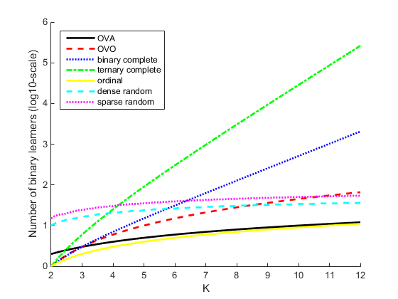
Coding Design	Description	Number of Learners	Minimal Pairwise Row Distance
one-versus-all (OVA)	For each binary learner, one class is positive and the rest are negative. This design exhausts all combinations of positive class assignments.	K	2
one-versus-one (OVO)	For each binary learner, one class is positive, another is negative, and the rest are ignored. This design exhausts all combinations of class pair assignments.	K(K – 1)/2	1
binary complete	This design partitions the classes into all binary combinations, and does not ignore any classes. That is, all class assignments are –1 and 1 with at least one positive class and one negative class in the assignment for each binary learner.	2K – 1 – 1	2K – 2
ternary complete	This design partitions the classes into all ternary combinations. That is, all class assignments are 0, –1, and 1 with at least one positive class and one negative class in the assignment for each binary learner.	(3K – 2K + 1 + 1)/2	3K – 2
ordinal	For the first binary learner, the first class is negative and the rest are positive. For the second binary learner, the first two classes are negative and the rest are positive, and so on.	K – 1	1
dense random	For each binary learner, the software randomly assigns classes into positive or negative classes, with at least one of each type. For more details, see Random Coding Design Matrices.	Random, but approximately 10 log2K	Variable
sparse random	For each binary learner, the software randomly assigns classes as positive or negative with probability 0.25 for each, and ignores classes with probability 0.5. For more details, see Random Coding Design Matrices.	Random, but approximately 15 log2K	Variable

This plot compares the number of binary learners for the coding designs with increasing K.

Error-Correcting Output Codes Model

An error-correcting output codes (ECOC) model reduces the problem of classification with three or more classes to a set of binary classification problems.

ECOC classification requires a coding design, which determines the classes that the binary learners train on, and a decoding scheme, which determines how the results (predictions) of the binary classifiers are aggregated.

Assume the following:

• The classification problem has three classes.

• The coding design is one-versus-one. For three classes, this coding design is

  $$\begin{array}{cccc}& \text{Learner 1}& \text{Learner 2}& \text{Learner 3}\\ \text{Class 1}& 1& 1& 0\\ \text{Class 2}& -1& 0& 1\\ \text{Class 3}& 0& -1& -1\end{array}$$

• The decoding scheme uses loss g.

• The learners are SVMs.

To build this classification model, the ECOC algorithm follows these steps.

1. Learner 1 trains on observations in Class 1 or Class 2, and treats Class 1 as the positive class and Class 2 as the negative class. The other learners are trained similarly.

2. Let M be the coding design matrix with elements m_kl, and s_l be the predicted classification score for the positive class of learner l. The algorithm assigns a new observation to the class ($$\widehat{k}$$) that minimizes the aggregation of the losses for the L binary learners.

   $$\widehat{k}=\underset{k}{\text{argmin}}\frac{{\displaystyle \sum }_{l=1}^L\left|m_{kl}\right|g\left(m_{kl},s_l\right)}{{\displaystyle \sum }_{l=1}^L\left|m_{kl}\right|}.$$

ECOC models can improve classification accuracy, compared to other multiclass models [2].

Tips

• The number of binary learners grows with the number of classes. For a problem with many classes, the binarycomplete and ternarycomplete coding designs are not efficient. However:

  • If K ≤ 4, then use ternarycomplete coding design rather than sparserandom.

  • If K ≤ 5, then use binarycomplete coding design rather than denserandom.

  You can display the coding design matrix of a trained ECOC classifier by entering Mdl.CodingMatrix into the Command Window.

• You should form a coding matrix using intimate knowledge of the application, and taking into account computational constraints. If you have sufficient computational power and time, then try several coding matrices and choose the one with the best performance (e.g., check the confusion matrices for each model using confusionchart).

• Leave-one-out cross-validation (Leaveout) is inefficient for data sets with many observations. Instead, use k-fold cross-validation (KFold).

• After training a model, you can generate C/C++ code that predicts labels for new data. Generating C/C++ code requires MATLAB Coder™. For details, see Introduction to Code Generation.

Algorithms

Custom Coding Design Matrices

Custom coding matrices must have a certain form. The software validates custom coding matrices by ensuring:

• Every element is -1, 0, or 1.

• Every column contains as least one -1 and one 1.

• For all distinct column vectors u and v, u ≠ v and u ≠ -v.

• All rows vectors are unique.

• The matrix can separate any two classes. That is, you can travel from any row to any other row following these rules:

  • You can move vertically from 1 to -1 or -1 to 1.

  • You can move horizontally from a nonzero element to another nonzero element.

  • You can use a column of the matrix for a vertical move only once.

  If it is not possible to move from row i to row j using these rules, then classes i and j cannot be separated by the design. For example, in the coding design

  $$\left[\begin{array}{cc}1& 0\\ -1& 0\\ 0& 1\\ 0& -1\end{array}\right]$$

  classes 1 and 2 cannot be separated from classes 3 and 4 (that is, you cannot move horizontally from the -1 in row 2 to column 2 since there is a 0 in that position). Therefore, the software rejects this coding design.

Parallel Computing

If you use parallel computing (see Options), then fitcecoc trains binary learners in parallel.

Prior Probabilities and Cost

• Prior probabilities — The software normalizes the specified class prior probabilities (Prior) for each binary learner. Let M be the coding design matrix and I(A,c) be an indicator matrix. The indicator matrix has the same dimensions as A. If the corresponding element of A is c, then the indicator matrix has elements equaling one, and zero otherwise. Let M₊₁ and M_-1 be K-by-L matrices such that:

  • M₊₁ = M○I(M,1), where ○ is element-wise multiplication (that is, Mplus = M.*(M == 1)). Also, let $$m_l^{(+1)}$$ be column vector l of M₊₁.

  • M_-1 = -M○I(M,-1) (that is, Mminus = -M.*(M == -1)). Also, let $$m_l^{(-1)}$$ be column vector l of M_-1.

  Let $${\pi }_l^{+1}=m_l^{(+1)}°\pi$$ and $${\pi }_l^{-1}=m_l^{(-1)}°\pi$$, where π is the vector of specified, class prior probabilities (Prior).

  Then, the positive and negative, scalar class prior probabilities for binary learner l are

  $${\widehat{\pi }}_l^{(j)}=\frac{{\Vert {\pi }_l^{(j)}\Vert }_1}{{\Vert {\pi }_l^{(+1)}\Vert }_1+{\Vert {\pi }_l^{(-1)}\Vert }_1},$$

  where j = {-1,1} and $${\Vert a\Vert }_1$$ is the one-norm of a.

• Cost — The software normalizes the K-by-K cost matrix C (Cost) for each binary learner. For binary learner l, the cost of classifying a negative-class observation into the positive class is

  $$c_l^{-+}={\left({\pi }_l^{(-1)}\right)}^{\top }C{\pi }_l^{(+1)}.$$

  Similarly, the cost of classifying a positive-class observation into the negative class is

  $$c_l^{+-}={\left({\pi }_l^{(+1)}\right)}^{\top }C{\pi }_l^{(-1)}.$$

  The cost matrix for binary learner l is

  $$C_l=\left[\begin{array}{cc}0& c_l^{-+}\\ c_l^{+-}& 0\end{array}\right].$$

  ECOC models accommodate misclassification costs by incorporating them with class prior probabilities. If you specify Prior and Cost, then the software adjusts the class prior probabilities as follows:

  $$\begin{array}{l}{\overline{\pi }}_l^{-1}=\frac{c_l^{-+}{\widehat{\pi }}_l^{-1}}{c_l^{-+}{\widehat{\pi }}_l^{-1}+c^{+-}{\widehat{\pi }}_l^{+1}}\\ {\overline{\pi }}_l^{+1}=\frac{c_l^{+-}{\widehat{\pi }}_l^{+1}}{c_l^{-+}{\widehat{\pi }}_l^{-1}+c^{+-}{\widehat{\pi }}_l^{+1}}.\end{array}$$

Random Coding Design Matrices

For a given number of classes K, the software generates random coding design matrices as follows.

1. The software generates one of these matrices:

   1. Dense random — The software assigns 1 or –1 with equal probability to each element of the K-by-L_d coding design matrix, where $$L_d\approx \lceil 10{\log }_{2}K\rceil$$.

   2. Sparse random — The software assigns 1 to each element of the K-by-L_s coding design matrix with probability 0.25, –1 with probability 0.25, and 0 with probability 0.5, where $$L_s\approx \lceil 15{\log }_{2}K\rceil$$.

2. If a column does not contain at least one 1 and at least one –1, then the software removes that column.

3. For distinct columns u and v, if u = v or u = –v, then the software removes v from the coding design matrix.

The software randomly generates 10,000 matrices by default, and retains the matrix with the largest, minimal, pairwise row distance based on the Hamming measure ([4]) given by

$$\Delta (k_1,k_2)=0.5{\displaystyle \sum }_{l=1}^L\left|m_{k_{1}l}\right|\left|m_{k_{2}l}\right|\left|m_{k_{1}l}-m_{k_{2}l}\right|,$$

where m_kjl is an element of coding design matrix j.

Support Vector Storage

By default and for efficiency, fitcecoc empties the Alpha, SupportVectorLabels, and SupportVectors properties for all linear SVM binary learners. fitcecoc lists Beta, rather than Alpha, in the model display.

To store Alpha, SupportVectorLabels, and SupportVectors, pass a linear SVM template that specifies storing support vectors to fitcecoc. For example, enter:

t = templateSVM('SaveSupportVectors',true)
Mdl = fitcecoc(X,Y,'Learners',t);

You can remove the support vectors and related values by passing the resulting ClassificationECOC model to discardSupportVectors.

References

[1] Allwein, E., R. Schapire, and Y. Singer. “Reducing multiclass to binary: A unifying approach for margin classifiers.” Journal of Machine Learning Research. Vol. 1, 2000, pp. 113–141.

[2] Fürnkranz, Johannes, “Round Robin Classification.” J. Mach. Learn. Res., Vol. 2, 2002, pp. 721–747.

[3] Escalera, S., O. Pujol, and P. Radeva. “On the decoding process in ternary error-correcting output codes.” IEEE Transactions on Pattern Analysis and Machine Intelligence. Vol. 32, Issue 7, 2010, pp. 120–134.

[4] Escalera, S., O. Pujol, and P. Radeva. “Separability of ternary codes for sparse designs of error-correcting output codes.” Pattern Recog. Lett., Vol. 30, Issue 3, 2009, pp. 285–297.

Extended Capabilities

Tall Arrays

Calculate with arrays that have more rows than fit in memory.

Usage notes and limitations:

• Supported syntaxes are:

  • Mdl = fitcecoc(X,Y)

  • Mdl = fitcecoc(X,Y,Name,Value)

  • [Mdl,FitInfo,HyperparameterOptimizationResults] = fitcecoc(X,Y,Name,Value) — fitcecoc returns the additional output arguments FitInfo and HyperparameterOptimizationResults when you specify the 'OptimizeHyperparameters' name-value pair argument.

• The FitInfo output argument is an empty structure array currently reserved for possible future use.

• Options related to cross-validation are not supported. The supported name-value pair arguments are:

  • 'ClassNames'

  • 'Cost'

  • 'Coding' — Default value is 'onevsall'.

  • 'HyperparameterOptimizationOptions' — For cross-validation, tall optimization supports only 'Holdout' validation. By default, the software selects and reserves 20% of the data as holdout validation data, and trains the model using the rest of the data. You can specify a different value for the holdout fraction by using this argument. For example, specify 'HyperparameterOptimizationOptions',struct('Holdout',0.3) to reserve 30% of the data as validation data.

  • 'Learners' — Default value is 'linear'. You can specify 'linear','kernel', a templateLinear or templateKernel object, or a cell array of such objects.

  • 'OptimizeHyperparameters' — When you use linear binary learners, the value of the 'Regularization' hyperparameter must be 'ridge'.

  • 'Prior'

  • 'Verbose' — Default value is 1.

  • 'Weights'

• This additional name-value pair argument is specific to tall arrays:

  • 'NumConcurrent' — A positive integer scalar specifying the number of binary learners that are trained concurrently by combining file I/O operations. The default value for 'NumConcurrent' is 1, which means fitcecoc trains the binary learners sequentially. 'NumConcurrent' is most beneficial when the input arrays cannot fit into the distributed cluster memory. Otherwise, the input arrays can be cached and speedup is negligible.

    If you run your code on Apache Spark™, NumConcurrent is upper bounded by the memory available for communications. Check the 'spark.executor.memory' and 'spark.driver.memory' properties in your Apache Spark configuration. See parallel.cluster.Hadoop (Parallel Computing Toolbox) for more details. For more information on Apache Spark and other execution environments that control where your code runs, see Extend Tall Arrays with Other Products.

For more information, see Tall Arrays.

Automatic Parallel Support

Accelerate code by automatically running computation in parallel using Parallel Computing Toolbox™.

To run in parallel, set the 'UseParallel' option to true in one of these ways:

• Set the 'UseParallel' field of the options structure to true using statset and specify the 'Options' name-value pair argument in the call to fitceoc.

  For example: 'Options',statset('UseParallel',true)

  For more information, see the 'Options' name-value pair argument.

• Perform parallel hyperparameter optimization by using the 'HyperparameterOptions',struct('UseParallel',true) name-value pair argument in the call to fitceoc.

  For more information on parallel hyperparameter optimization, see Parallel Bayesian Optimization.

GPU Arrays

Accelerate code by running on a graphics processing unit (GPU) using Parallel Computing Toolbox™.

Usage notes and limitations:

• You can specify the name-value argument 'Learners' only as one of the learners specified in this table.

  Learner	Learner Name	Template Object Creation Function	Information About gpuArray Support
  support vector machine	'svm'	templateSVM	GPU Arrays for fitcsvm
  k-nearest neighbors	'knn'	templateKNN	GPU Arrays for fitcknn
  classification tree	'tree'	templateTree	GPU Arrays for fitctree

For more information, see Run MATLAB Functions on a GPU (Parallel Computing Toolbox).