confusionchart
Create confusion matrix chart for classification problem
Syntax
Description
confusionchart( creates a confusion matrix chart from true labels trueLabels,predictedLabels)trueLabels and predicted labels predictedLabels and returns a ConfusionMatrixChart object. The rows of the confusion matrix correspond to the true class and the columns correspond to the predicted class. Diagonal and off-diagonal cells correspond to correctly and incorrectly classified observations, respectively. Use cm to modify the confusion matrix chart after it is created. For a list of properties, see ConfusionMatrixChart Properties.
confusionchart( creates a confusion matrix chart from the numeric confusion matrix m)m. Use this syntax if you already have a numeric confusion matrix in the workspace.
confusionchart( specifies class labels that appear along the x-axis and y-axis. Use this syntax if you already have a numeric confusion matrix and class labels in the workspace.m,classLabels)
confusionchart( creates the confusion chart in the figure, panel, or tab specified by parent,___)parent.
confusionchart(___, specifies additional Name,Value)ConfusionMatrixChart properties using one or more name-value pair arguments. Specify the properties after all other input arguments. For a list of properties, see ConfusionMatrixChart Properties.
cm = confusionchart(___)ConfusionMatrixChart object. Use cm to modify properties of the chart after creating it. For a list of properties, see ConfusionMatrixChart Properties.
Examples
Load Fisher's iris data set.
load fisheriris
X = meas;
Y = species;
X is a numeric matrix that contains four measurements for 150 irises. Y is a cell array of character vectors that contains the corresponding iris species.
Train a k-nearest neighbor (KNN) classifier, where the number of nearest neighbors in the predictors (k) is 5. A good practice is to standardize numeric predictor data.
Mdl = fitcknn(X,Y,'NumNeighbors',5,'Standardize',1);
Predict the labels of the training data.
predictedY = resubPredict(Mdl);
Create a confusion matrix chart from the true labels Y and the predicted labels predictedY.
cm = confusionchart(Y,predictedY);
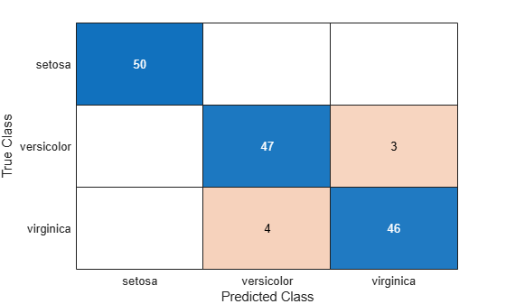
The confusion matrix displays the total number of observations in each cell. The rows of the confusion matrix correspond to the true class, and the columns correspond to the predicted class. Diagonal and off-diagonal cells correspond to correctly and incorrectly classified observations, respectively.
By default, confusionchart sorts the classes into their natural order as defined by sort. In this example, the class labels are character vectors, so confusionchart sorts the classes alphabetically. Use sortClasses to sort the classes by a specified order or by the confusion matrix values.
The NormalizedValues property contains the values of the confusion matrix. Display these values using dot notation.
cm.NormalizedValues
ans = 3×3

    50     0     0
     0    47     3
     0     4    46
Modify the appearance and behavior of the confusion matrix chart by changing property values. Add a title.
cm.Title = 'Iris Flower Classification Using KNN';Add column and row summaries.
cm.RowSummary = 'row-normalized';
cm.ColumnSummary = 'column-normalized';
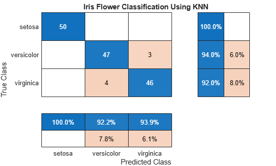
A row-normalized row summary displays the percentages of correctly and incorrectly classified observations for each true class. A column-normalized column summary displays the percentages of correctly and incorrectly classified observations for each predicted class.
Create a confusion matrix chart and sort the classes of the chart according to the class-wise true positive rate (recall) or the class-wise positive predictive value (precision).
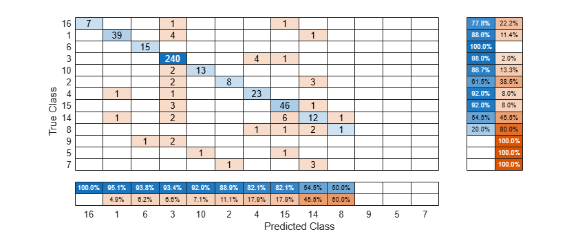
Load and inspect the arrhythmia data set.
load arrhythmia
isLabels = unique(Y);
nLabels = numel(isLabels)
nLabels = 13
tabulate(categorical(Y))
  Value    Count   Percent
      1      245     54.20%
      2       44      9.73%
      3       15      3.32%
      4       15      3.32%
      5       13      2.88%
      6       25      5.53%
      7        3      0.66%
      8        2      0.44%
      9        9      1.99%
     10       50     11.06%
     14        4      0.88%
     15        5      1.11%
     16       22      4.87%
The data contains 16 distinct labels that describe various degrees of arrhythmia, but the response (Y) includes only 13 distinct labels.
Train a classification tree and predict the resubstitution response of the tree.
Mdl = fitctree(X,Y);
predictedY = resubPredict(Mdl);
Create a confusion matrix chart from the true labels Y and the predicted labels predictedY. Specify 'RowSummary' as 'row-normalized' to display the true positive rates and false positive rates in the row summary. Also, specify 'ColumnSummary' as 'column-normalized' to display the positive predictive values and false discovery rates in the column summary.
fig = figure;
cm = confusionchart(Y,predictedY,'RowSummary','row-normalized','ColumnSummary','column-normalized');
Resize the container of the confusion chart so percentages appear in the row summary.
fig_Position = fig.Position;
fig_Position(3) = fig_Position(3)*1.5;
fig.Position = fig_Position;
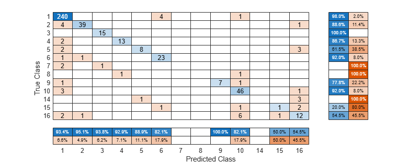
To sort the confusion matrix according to the true positive rate, normalize the cell values across each row by setting the Normalization property to 'row-normalized' and then use sortClasses. After sorting, reset the Normalization property back to 'absolute' to display the total number of observations in each cell.
cm.Normalization = 'row-normalized';
sortClasses(cm,'descending-diagonal')
cm.Normalization = 'absolute';
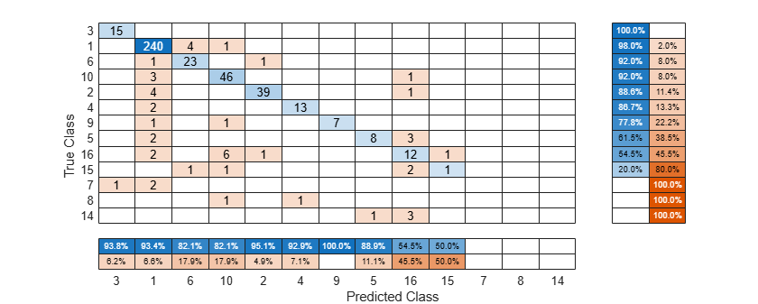
To sort the confusion matrix according to the positive predictive value, normalize the cell values across each column by setting the Normalization property to 'column-normalized' and then use sortClasses. After sorting, reset the Normalization property back to 'absolute' to display the total number of observations in each cell.
cm.Normalization = 'column-normalized';
sortClasses(cm,'descending-diagonal')
cm.Normalization = 'absolute';
Perform classification on a tall array of the Fisher iris data set. Compute a confusion matrix chart for the known and predicted tall labels by using the confusionchart function.
When you perform calculations on tall arrays, MATLAB® uses either a parallel pool (default if you have Parallel Computing Toolbox™) or the local MATLAB session. To run the example using the local MATLAB session when you have Parallel Computing Toolbox, change the global execution environment by using the mapreducer function.
mapreducer(0)
Load Fisher's iris data set.
load fisheririsConvert the in-memory arrays meas and species to tall arrays.
tx = tall(meas);
ty = tall(species);
Find the number of observations in the tall array.
numObs = gather(length(ty)); % gather collects tall array into memorySet the seeds of the random number generators using rng and tallrng for reproducibility, and randomly select training samples. The results can vary depending on the number of workers and the execution environment for the tall arrays. For details, see Control Where Your Code Runs.
rng('default')
tallrng('default')
numTrain = floor(numObs/2);
[txTrain,trIdx] = datasample(tx,numTrain,'Replace',false);
tyTrain = ty(trIdx);
Fit a decision tree classifier model on the training samples.
mdl = fitctree(txTrain,tyTrain);
Evaluating tall expression using the Local MATLAB Session:
- Pass 1 of 2: Completed in 0.39 sec
- Pass 2 of 2: Completed in 0.38 sec
Evaluation completed in 1.2 sec
Evaluating tall expression using the Local MATLAB Session:
- Pass 1 of 4: Completed in 0.19 sec
- Pass 2 of 4: Completed in 0.25 sec
- Pass 3 of 4: Completed in 0.35 sec
- Pass 4 of 4: Completed in 0.31 sec
Evaluation completed in 1.3 sec
Evaluating tall expression using the Local MATLAB Session:
- Pass 1 of 4: Completed in 0.072 sec
- Pass 2 of 4: Completed in 0.075 sec
- Pass 3 of 4: Completed in 0.14 sec
- Pass 4 of 4: Completed in 0.14 sec
Evaluation completed in 0.53 sec
Evaluating tall expression using the Local MATLAB Session:
- Pass 1 of 4: Completed in 0.12 sec
- Pass 2 of 4: Completed in 0.13 sec
- Pass 3 of 4: Completed in 0.11 sec
- Pass 4 of 4: Completed in 0.093 sec
Evaluation completed in 0.56 sec
Evaluating tall expression using the Local MATLAB Session:
- Pass 1 of 4: Completed in 0.15 sec
- Pass 2 of 4: Completed in 0.064 sec
- Pass 3 of 4: Completed in 0.15 sec
- Pass 4 of 4: Completed in 0.071 sec
Evaluation completed in 0.53 sec
Predict labels for the test samples by using the trained model.
txTest = tx(~trIdx,:);
label = predict(mdl,txTest);
Create the confusion matrix chart for the resulting classification.
tyTest = ty(~trIdx);
cm = confusionchart(tyTest,label)
Evaluating tall expression using the Local MATLAB Session:
- Pass 1 of 1: Completed in 0.077 sec
Evaluation completed in 0.2 sec
Evaluating tall expression using the Local MATLAB Session:
- Pass 1 of 1: Completed in 0.15 sec
Evaluation completed in 0.23 sec
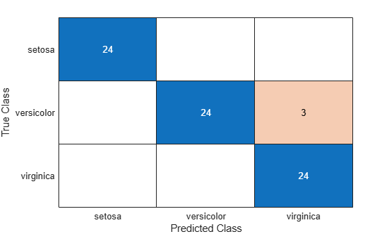
cm =
  ConfusionMatrixChart with properties:

    NormalizedValues: [3×3 double]
         ClassLabels: {3×1 cell}

  Show all properties
The confusion matrix chart shows that three measurements in the versicolor class are misclassified. All the measurements belonging to setosa and virginica are classified correctly.
Input Arguments
Name-Value Arguments
Output Arguments
Limitations
MATLAB® code generation is not supported for
ConfusionMatrixChartobjects.