ss

State-space model

Description

Use ss to create real-valued or complex-valued state-space models, or to convert dynamic system models to state-space model form. You can also use ss to create generalized state-space (genss) models or uncertain state-space (uss (Robust Control Toolbox)) models.

A state-space model is a mathematical representation of a physical system as a set of input, output, and state variables related by first-order differential equations. The state variables define the values of the output variables. The ss model object can represent SISO or MIMO state-space models in continuous time or discrete time.

In continuous-time, a state-space model is of the following form:

$$\begin{array}{l}\dot{x}=Ax+Bu\\ y=Cx+Du\end{array}$$

Here, x, u and y represent the states, inputs and outputs respectively, while A, B, C and D are the state-space matrices. The ss object represents a state-space model in MATLAB^® storing A, B, C and D along with other information such as sample time, names and delays specific to the inputs and outputs.

You can create a state-space model object by either specifying the state, input and output matrices directly, or by converting a model of another type (such as a transfer function model tf) to state-space form. For more information, see State-Space Models. You can use an ss model object to:

• Perform linear analysis

• Represent a linear time-invariant (LTI) model to perform control design

• Combine with other LTI models to represent a more complex system

Creation

Syntax

sys = ss(A,B,C,D)

sys = ss(A,B,C,D,ts)

sys = ss(A,B,C,D,ltiSys)

sys = ss(D)

sys = ss(___,Name,Value)

sys = ss(ltiSys)

sys = ss(ltiSys,component)

sys = ss(ssSys,'minimal')

sys = ss(ssSys,'explicit')

Description

sys = ss(A,B,C,D) creates a continuous-time state-space model object of the following form:

$$\begin{array}{l}\dot{x}=Ax+Bu\\ y=Cx+Du\end{array}$$

For instance, consider a plant with Nx states, Ny outputs, and Nu inputs. The state-space matrices are:

• A is an Nx-by-Nx real- or complex-valued matrix.

• B is an Nx-by-Nu real- or complex-valued matrix.

• C is an Ny-by-Nx real- or complex-valued matrix.

• D is an Ny-by-Nu real- or complex-valued matrix.

sys = ss(A,B,C,D,ts) creates the discrete-time state-space model object of the following form with the sample time ts (in seconds):

$$\begin{array}{l}x[n+1]=Ax[n]+Bu[n]\\ y[n]=Cx[n]+Du[n]\end{array}$$

To leave the sample time unspecified, set ts to -1.

sys = ss(A,B,C,D,ltiSys) creates a state-space model with properties such as input and output names, internal delays and sample time values inherited from the model ltisys.

sys = ss(D) creates a state-space model that represents the static gain, D. The output state-space model is equivalent to ss([],[],[],D).

sys = ss(___,Name,Value) sets properties of the state-space model using one or more Name,Value pair arguments for any of the previous input-argument combinations.

sys = ss(ltiSys) converts the dynamic system model ltiSys to a state-space model. If ltiSys contains tunable or uncertain elements, ss uses the current or nominal values for those elements respectively.

sys = ss(ltiSys,component) converts to ss object form the measured component, the noise component or both of specified component of an identified linear time-invariant (LTI) model ltiSys. Use this syntax only when ltiSys is an identified (LTI) model such as an idtf (System Identification Toolbox), idss (System Identification Toolbox), idproc (System Identification Toolbox), idpoly (System Identification Toolbox) or idgrey (System Identification Toolbox) object.

sys = ss(ssSys,'minimal') returns the minimal state-space realization with no uncontrollable or unobservable states. This realization is equivalent to minreal(ss(sys)) where matrix A has the smallest possible dimension.

Conversion to state-space form is not uniquely defined in the SISO case. It is also not guaranteed to produce a minimal realization in the MIMO case. For more information, see Recommended Working Representation.

sys = ss(ssSys,'explicit') returns an explicit state-space realization (E = I) of the dynamic system state-space model ssSys. ss returns an error if ssSys is improper. For more information on explicit state-space realization, see State-Space Models.

Input Arguments

A — State matrix

Nx-by-Nx matrix

State matrix, specified as an Nx-by-Nx matrix where, Nx is the number of states. This input sets the value of property A.

B — Input-to-state matrix

Nx-by-Nu matrix

Input-to-state matrix, specified as an Nx-by-Nu matrix where, Nx is the number of states and Nu is the number of inputs. This input sets the value of property B.

C — State-to-output matrix

Ny-by-Nx matrix

State-to-output matrix, specified as an Ny-by-Nx matrix where, Nx is the number of states and Ny is the number of outputs. This input sets the value of property C.

D — Feedthrough matrix

Ny-by-Nu matrix

Feedthrough matrix, specified as an Ny-by-Nu matrix where, Ny is the number of outputs and Nu is the number of inputs. This input sets the value of property D.

ts — Sample time

scalar

Sample time, specified as a scalar. For more information, see Ts property.

ltiSys — Dynamic system to convert to state-space form

dynamic system model | model array

Dynamic system to convert to state-space form, specified as a SISO or MIMO dynamic system model or array of dynamic system models. Dynamic systems that you can convert include:

• Continuous-time or discrete-time numeric LTI models, such as tf, zpk, ss, or pid models.

• Generalized or uncertain LTI models such as genss or uss (Robust Control Toolbox) models. (Using uncertain models requires Robust Control Toolbox™ software.)

  The resulting state-space model assumes

  • current values of the tunable components for tunable control design blocks.

  • nominal model values for uncertain control design blocks.

• Identified LTI models, such as idtf (System Identification Toolbox), idss (System Identification Toolbox), idproc (System Identification Toolbox), idpoly (System Identification Toolbox), and idgrey (System Identification Toolbox) models. To select the component of the identified model to convert, specify component. If you do not specify component, ss converts the measured component of the identified model by default. (Using identified models requires System Identification Toolbox™ software.)

component — Component of identified model

'measured' (default) | 'noise' | 'augmented'

Component of identified model to convert, specified as one of the following:

• 'measured' — Convert the measured component of sys.

• 'noise' — Convert the noise component of sys

• 'augmented' — Convert both the measured and noise components of sys.

component only applies when sys is an identified LTI model.

For more information on identified LTI models and their measured and noise components, see Identified LTI Models.

ssSys — Dynamic system model to convert to minimal realization or explicit form

ss model object

Dynamic system model to convert to minimal realization or explicit form, specified as an ss model object.

Output Arguments

sys — Output system model

ss model object | genss model object | uss model object

Output system model, returned as:

• A state-space (ss) model object, when the inputs A, B, C and D are numeric matrices or when converting from another model object type.

• A generalized state-space model (genss) object, when one or more of the matrices A, B, C and D includes tunable parameters, such as realp parameters or generalized matrices (genmat). For an example, see Create State-Space Model with Both Fixed and Tunable Parameters.

• An uncertain state-space model (uss) object, when one or more of the inputs A, B, C and D includes uncertain matrices. Using uncertain models requires Robust Control Toolbox software.

Properties

A — State matrix

Nx-by-Nx matrix

State matrix, specified as an Nx-by-Nx matrix where Nx is the number of states. The state-matrix can be represented in many ways depending on the desired state-space model realization such as:

• Model Canonical Form

• Companion Canonical Form

• Observable Canonical Form

• Controllable Canonical Form

For more information, see State-Space Realizations.

B — Input-to-state matrix

Nx-by-Nu matrix

Input-to-state matrix, specified as an Nx-by-Nu matrix where Nx is the number of states and Nu is the number of inputs.

C — State-to-output matrix

Ny-by-Nx matrix

State-to-output matrix, specified as an Ny-by-Nx matrix where Nx is the number of states and Ny is the number of outputs.

D — Feedthrough matrix

Ny-by-Nu matrix

Feedthrough matrix, specified as an Ny-by-Nu matrix where Ny is the number of outputs and Nu is the number of inputs. D is also called as the static gain matrix which represents the ratio of the output to the input under steady state condition.

E — Matrix for implicit state-space models

[] (default) | Nx-by-Nx matrix

Matrix for implicit or descriptor state-space models, specified as a Nx-by-Nx matrix. E is empty by default, meaning that the state equation is explicit. To specify an implicit state equation E dx/dt = Ax + Bu, set this property to a square matrix of the same size as A. See dss for more information about creating descriptor state-space models.

Scaled — Logical value indicating whether scaling is enabled or disabled

0 (default) | 1

Logical value indicating whether scaling is enabled or disabled, specified as either 0 or 1.

When Scaled is set to 0 (disabled), then most numerical algorithms acting on the state-space model sys automatically rescale the state vector to improve numerical accuracy. You can prevent such auto-scaling by setting Scaled to 1 (enabled).

For more information about scaling, see prescale.

StateName — State names

' ' (default) | character vector | cell array of character vectors

State names, specified as one of the following:

• Character vector — For first-order models, for example, 'velocity'

• Cell array of character vectors — For models with two or more states

StateName is empty ' ' for all states by default.

StatePath — State path

' ' (default) | character vector | cell array of character vectors

State path to facilitate state block path management in linearization, specified as one of the following:

• Character vector — For first-order models

• Cell array of character vectors — For models with two or more states

StatePath is empty ' ' for all states by default.

StateUnit — State units

' ' (default) | character vector | cell array of character vectors

State units, specified as one of the following:

• Character vector — For first-order models, for example, 'm/s'

• Cell array of character vectors — For models with two or more states

Use StateUnit to keep track of the units of each state. StateUnit has no effect on system behavior. StateUnit is empty ' ' for all states by default.

InternalDelay — Internal delays in the model

vector

Internal delays in the model, specified as a vector. Internal delays arise, for example, when closing feedback loops on systems with delays, or when connecting delayed systems in series or parallel. For more information about internal delays, see Closing Feedback Loops with Time Delays.

For continuous-time models, internal delays are expressed in the time unit specified by the TimeUnit property of the model. For discrete-time models, internal delays are expressed as integer multiples of the sample time Ts. For example, InternalDelay = 3 means a delay of three sampling periods.

You can modify the values of internal delays using the property InternalDelay. However, the number of entries in sys.InternalDelay cannot change, because it is a structural property of the model.

InputDelay — Input delay

0 (default) | scalar | Nu-by-1 vector

Input delay for each input channel, specified as one of the following:

• Scalar — Specify the input delay for a SISO system or the same delay for all inputs of a multi-input system.

• Nu-by-1 vector — Specify separate input delays for input of a multi-input system, where Nu is the number of inputs.

For continuous-time systems, specify input delays in the time unit specified by the TimeUnit property. For discrete-time systems, specify input delays in integer multiples of the sample time, Ts.

For more information, see Time Delays in Linear Systems.

OutputDelay — Output delay

0 (default) | scalar | Ny-by-1 vector

Output delay for each output channel, specified as one of the following:

• Scalar — Specify the output delay for a SISO system or the same delay for all outputs of a multi-output system.

• Ny-by-1 vector — Specify separate output delays for output of a multi-output system, where Ny is the number of outputs.

For continuous-time systems, specify output delays in the time unit specified by the TimeUnit property. For discrete-time systems, specify output delays in integer multiples of the sample time, Ts.

For more information, see Time Delays in Linear Systems.

Ts — Sample time

0 (default) | positive scalar | -1

Sample time, specified as:

• 0 for continuous-time systems.

• A positive scalar representing the sampling period of a discrete-time system. Specify Ts in the time unit specified by the TimeUnit property.

• -1 for a discrete-time system with an unspecified sample time.

Note

Changing Ts does not discretize or resample the model. To convert between continuous-time and discrete-time representations, use c2d and d2c. To change the sample time of a discrete-time system, use d2d.

TimeUnit — Time variable units

'seconds' (default) | 'nanoseconds' | 'microseconds' | 'milliseconds' | 'minutes' | 'hours' | 'days' | 'weeks' | 'months' | 'years' | ...

Time variable units, specified as one of the following:

• 'nanoseconds'

• 'microseconds'

• 'milliseconds'

• 'seconds'

• 'minutes'

• 'hours'

• 'days'

• 'weeks'

• 'months'

• 'years'

Changing TimeUnit has no effect on other properties, but changes the overall system behavior. Use chgTimeUnit to convert between time units without modifying system behavior.

InputName — Input channel names

'' (default) | character vector | cell array of character vectors

Input channel names, specified as one of the following:

• A character vector, for single-input models.

• A cell array of character vectors, for multi-input models.

• '', no names specified, for any input channels.

Alternatively, you can assign input names for multi-input models using automatic vector expansion. For example, if sys is a two-input model, enter the following:

sys.InputName = 'controls';

The input names automatically expand to {'controls(1)';'controls(2)'}.

You can use the shorthand notation u to refer to the InputName property. For example, sys.u is equivalent to sys.InputName.

Use InputName to:

• Identify channels on model display and plots.

• Extract subsystems of MIMO systems.

• Specify connection points when interconnecting models.

InputUnit — Input channel units

'' (default) | character vector | cell array of character vectors

Input channel units, specified as one of the following:

• A character vector, for single-input models.

• A cell array of character vectors, for multi-input models.

• '', no units specified, for any input channels.

Use InputUnit to specify input signal units. InputUnit has no effect on system behavior.

InputGroup — Input channel groups

structure

Input channel groups, specified as a structure. Use InputGroup to assign the input channels of MIMO systems into groups and refer to each group by name. The field names of InputGroup are the group names and the field values are the input channels of each group. For example, enter the following to create input groups named controls and noise that include input channels 1 and 2, and 3 and 5, respectively.

sys.InputGroup.controls = [1 2];
sys.InputGroup.noise = [3 5];

You can then extract the subsystem from the controls inputs to all outputs using the following.

sys(:,'controls')

By default, InputGroup is a structure with no fields.

OutputName — Output channel names

'' (default) | character vector | cell array of character vectors

Output channel names, specified as one of the following:

• A character vector, for single-output models.

• A cell array of character vectors, for multi-output models.

• '', no names specified, for any output channels.

Alternatively, you can assign output names for multi-output models using automatic vector expansion. For example, if sys is a two-output model, enter the following.

sys.OutputName = 'measurements';

The output names automatically expand to {'measurements(1)';'measurements(2)'}.

You can also use the shorthand notation y to refer to the OutputName property. For example, sys.y is equivalent to sys.OutputName.

Use OutputName to:

• Identify channels on model display and plots.

• Extract subsystems of MIMO systems.

• Specify connection points when interconnecting models.

OutputUnit — Output channel units

'' (default) | character vector | cell array of character vectors

Output channel units, specified as one of the following:

• A character vector, for single-output models.

• A cell array of character vectors, for multi-output models.

• '', no units specified, for any output channels.

Use OutputUnit to specify output signal units. OutputUnit has no effect on system behavior.

OutputGroup — Output channel groups

structure

Output channel groups, specified as a structure. Use OutputGroupto assign the output channels of MIMO systems into groups and refer to each group by name. The field names of OutputGroup are the group names and the field values are the output channels of each group. For example, create output groups named temperature and measurement that include output channels 1, and 3 and 5, respectively.

sys.OutputGroup.temperature = [1];
sys.OutputGroup.measurement = [3 5];

You can then extract the subsystem from all inputs to the measurement outputs using the following.

sys('measurement',:)

By default, OutputGroup is a structure with no fields.

Name — System name

'' (default) | character vector

System name, specified as a character vector. For example, 'system_1'.

Notes — User-specified text

{} (default) | character vector | cell array of character vectors

User-specified text that you want to associate with the system, specified as a character vector or cell array of character vectors. For example, 'System is MIMO'.

UserData — User-specified data

[] (default) | any MATLAB data type

User-specified data that you want to associate with the system, specified as any MATLAB data type.

SamplingGrid — Sampling grid for model arrays

structure array

Sampling grid for model arrays, specified as a structure array.

Use SamplingGrid to track the variable values associated with each model in a model array, including identified linear time-invariant (IDLTI) model arrays.

Set the field names of the structure to the names of the sampling variables. Set the field values to the sampled variable values associated with each model in the array. All sampling variables must be numeric scalars, and all arrays of sampled values must match the dimensions of the model array.

For example, you can create an 11-by-1 array of linear models, sysarr, by taking snapshots of a linear time-varying system at times t = 0:10. The following code stores the time samples with the linear models.

 sysarr.SamplingGrid = struct('time',0:10)

Similarly, you can create a 6-by-9 model array, M, by independently sampling two variables, zeta and w. The following code maps the (zeta,w) values to M.

[zeta,w] = ndgrid(<6 values of zeta>,<9 values of w>)
M.SamplingGrid = struct('zeta',zeta,'w',w)

When you display M, each entry in the array includes the corresponding zeta and w values.

M

M(:,:,1,1) [zeta=0.3, w=5] =
 
        25
  --------------
  s^2 + 3 s + 25
 

M(:,:,2,1) [zeta=0.35, w=5] =
 
         25
  ----------------
  s^2 + 3.5 s + 25
 
...

For model arrays generated by linearizing a Simulink^® model at multiple parameter values or operating points, the software populates SamplingGrid automatically with the variable values that correspond to each entry in the array. For instance, the Simulink Control Design™ commands linearize (Simulink Control Design) and slLinearizer (Simulink Control Design) populate SamplingGrid automatically.

By default, SamplingGrid is a structure with no fields.

Object Functions

The following lists contain a representative subset of the functions you can use with ss model objects. In general, any function applicable to Dynamic System Models is applicable to an ss object.

Linear Analysis

step	Step response plot of dynamic system; step response data
impulse	Impulse response plot of dynamic system; impulse response data
lsim	Plot simulated time response of dynamic system to arbitrary inputs; simulated response data
bode	Bode plot of frequency response, or magnitude and phase data
nyquist	Nyquist plot of frequency response
nichols	Nichols chart of frequency response
bandwidth	Frequency response bandwidth

Stability Analysis

pole	Poles of dynamic system
zero	Zeros and gain of SISO dynamic system
pzplot	Pole-zero plot of dynamic system model with additional plot customization options
margin	Gain margin, phase margin, and crossover frequencies

Model Transformation

zpk	Zero-pole-gain model
tf	Transfer function model
c2d	Convert model from continuous to discrete time
d2c	Convert model from discrete to continuous time
d2d	Resample discrete-time model

Model Interconnection

feedback	Feedback connection of multiple models
connect	Block diagram interconnections of dynamic systems
series	Series connection of two models
parallel	Parallel connection of two models

Controller Design

pidtune	PID tuning algorithm for linear plant model
rlocus	Root locus plot of dynamic system
lqr	Linear-Quadratic Regulator (LQR) design
lqg	Linear-Quadratic-Gaussian (LQG) design
lqi	Linear-Quadratic-Integral control
kalman	Design Kalman filter for state estimation

Examples

SISO State-Space Model

Create the SISO state-space model defined by the following state-space matrices:

$$A=\left[\begin{array}{cc}-1.5& -2\\ 1& 0\end{array}\right]B=\left[\begin{array}{c}0.5\\ 0\end{array}\right]C=\left[\begin{array}{cc}0& 1\end{array}\right]D=0$$

Specify the A, B, C and D matrices, and create the state-space model.

A = [-1.5,-2;1,0];
B = [0.5;0];
C = [0,1];
D = 0;
sys = ss(A,B,C,D)

sys =
 
  A = 
         x1    x2
   x1  -1.5    -2
   x2     1     0
 
  B = 
        u1
   x1  0.5
   x2    0
 
  C = 
       x1  x2
   y1   0   1
 
  D = 
       u1
   y1   0
 
Continuous-time state-space model.

Create Discrete-Time State-Space Model

Create a state-space model with a sample time of 0.25 seconds and the following state-space matrices:

$$A=\left[\begin{array}{cc}0& 1\\ -5& -2\end{array}\right]B=\left[\begin{array}{c}0\\ 3\end{array}\right]C=[\begin{array}{cc}0& 1\end{array}]D=[0]$$

Specify the state-space matrices.

A = [0 1;-5 -2];
B = [0;3];
C = [0 1];
D = 0;

Specify the sample time.

Ts = 0.25;

Create the state-space model.

sys = ss(A,B,C,D,Ts);

Continuous-Time MIMO State-Space Model

For this example, consider a cube rotating about its corner with inertia tensor J and a damping force F of 0.2 magnitude. The input to the system is the driving torque while the angular velocities are the outputs. The state-space matrices for the cube are:

$$\begin{array}{l}A=-J^{-1}F,B=J^{-1},C=I,D=0,\\ where,J=\left[\begin{array}{ccc}8& -3& -3\\ -3& 8& -3\\ -3& -3& 8\end{array}\right]andF=\left[\begin{array}{ccc}0.2& 0& 0\\ 0& 0.2& 0\\ 0& 0& 0.2\end{array}\right]\end{array}$$

Specify the A, B, C and D matrices, and create the continuous-time state-space model.

J = [8 -3 -3; -3 8 -3; -3 -3 8];
F = 0.2*eye(3);
A = -J\F;
B = inv(J);
C = eye(3);
D = 0;
sys = ss(A,B,C,D)

sys =
 
  A = 
             x1        x2        x3
   x1  -0.04545  -0.02727  -0.02727
   x2  -0.02727  -0.04545  -0.02727
   x3  -0.02727  -0.02727  -0.04545
 
  B = 
           u1      u2      u3
   x1  0.2273  0.1364  0.1364
   x2  0.1364  0.2273  0.1364
   x3  0.1364  0.1364  0.2273
 
  C = 
       x1  x2  x3
   y1   1   0   0
   y2   0   1   0
   y3   0   0   1
 
  D = 
       u1  u2  u3
   y1   0   0   0
   y2   0   0   0
   y3   0   0   0
 
Continuous-time state-space model.

sys is MIMO since the system contains 3 inputs and 3 outputs observed from matrices C and D. For more information on MIMO state-space models, see MIMO State-Space Models.

Discrete-Time MIMO State-Space Model

Create a state-space model using the following discrete-time, multi-input, multi-output state matrices with sample time ts = 0.2 seconds:

$$A=\left[\begin{array}{cc}-7& 0\\ 0& -10\end{array}\right]B=\left[\begin{array}{cc}5& 0\\ 0& 2\end{array}\right]C=\left[\begin{array}{cc}1& -4\\ -4& 0.5\end{array}\right]D=\left[\begin{array}{cc}0& -2\\ 2& 0\end{array}\right]$$

Specify the state-space matrices and create the discrete-time MIMO state-space model.

A = [-7,0;0,-10];
B = [5,0;0,2];
C = [1,-4;-4,0.5];
D = [0,-2;2,0];
ts = 0.2;
sys = ss(A,B,C,D,ts)

sys =
 
  A = 
        x1   x2
   x1   -7    0
   x2    0  -10
 
  B = 
       u1  u2
   x1   5   0
   x2   0   2
 
  C = 
        x1   x2
   y1    1   -4
   y2   -4  0.5
 
  D = 
       u1  u2
   y1   0  -2
   y2   2   0
 
Sample time: 0.2 seconds
Discrete-time state-space model.

Specify State and Input Names for State-Space Model

Create state-space matrices and specify sample time.

A = [0 1;-5 -2];
B = [0;3];
C = [0 1];
D = 0;
Ts = 0.05;

Create the state-space model, specifying the state and input names using name-value pairs.

sys = ss(A,B,C,D,Ts,'StateName',{'Position' 'Velocity'},...
    'InputName','Force');

The number of state and input names must be consistent with the dimensions of A, B, C, and D.

Naming the inputs and outputs can be useful when dealing with response plots for MIMO systems.

step(sys)

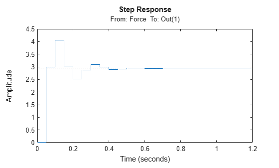
Notice the input name Force in the title of the step response plot.

State-Space Model with Inherited Properties

For this example, create a state-space model with the same time and input unit properties inherited from another state-space model. Consider the following state-space models:

$$\begin{array}{l}{A}_1=\left[\begin{array}{cc}-1.5& -2\\ 1& 0\end{array}\right]B_1=\left[\begin{array}{c}0.5\\ 0\end{array}\right]C_1=\left[\begin{array}{cc}0& 1\end{array}\right]D_1=5\\ A_2=\left[\begin{array}{cc}7& -1\\ 0& 2\end{array}\right]B_2=\left[\begin{array}{c}0.85\\ 2\end{array}\right]C_2=\left[\begin{array}{cc}10& 14\end{array}\right]D_2=2\end{array}$$

First, create a state-space model sys1 with the TimeUnit and InputUnit property set to 'minutes'.

A1 = [-1.5,-2;1,0];
B1 = [0.5;0];
C1 = [0,1];
D1 = 5;
sys1 = ss(A1,B1,C1,D1,'TimeUnit','minutes','InputUnit','minutes');

Verify that the time and input unit properties of sys1 are set to 'minutes'.

propValues1 = [sys1.TimeUnit,sys1.InputUnit]

propValues1 = 1x2 cell
    {'minutes'}    {'minutes'}

Create the second state-space model with properties inherited from sys1.

A2 = [7,-1;0,2];
B2 = [0.85;2];
C2 = [10,14];
D2 = 2;
sys2 = ss(A2,B2,C2,D2,sys1);

Verify that the time and input units of sys2 have been inherited from sys1.

propValues2 = [sys2.TimeUnit,sys2.InputUnit]

propValues2 = 1x2 cell
    {'minutes'}    {'minutes'}

MIMO Static Gain State-Space Model

In this example, you will create a static gain MIMO state-space model.

Consider the following two-input, two-output static gain matrix:

$$D=\left[\begin{array}{cc}2& 4\\ 3& 5\end{array}\right]$$

Specify the gain matrix and create the static gain state-space model.

D = [2,4;3,5];
sys1 = ss(D)

sys1 =
 
  D = 
       u1  u2
   y1   2   4
   y2   3   5
 
Static gain.

Convert Transfer Function to State-Space Model

Compute the state-space model of the following transfer function:

$$H\left(s\right)=\left[\begin{array}{c}\frac{s+1}{s^3+3s^2+3s+2}\\ \frac{s^2+3}{s^2+s+1}\end{array}\right]$$

Create the transfer function model.

H = [tf([1 1],[1 3 3 2]) ; tf([1 0 3],[1 1 1])];

Convert this model to a state-space model.

sys = ss(H);

Examine the size of the state-space model.

size(sys)

State-space model with 2 outputs, 1 inputs, and 5 states.

The number of states is equal to the cumulative order of the SISO entries in H(s).

To obtain a minimal realization of H(s), enter

sys = ss(H,'minimal');
size(sys)

State-space model with 2 outputs, 1 inputs, and 3 states.

The resulting model has an order of three, which is the minimum number of states needed to represent H(s). To see this number of states, refactor H(s) as the product of a first-order system and a second-order system.

$$H(s)=\left[\begin{array}{cc}\frac{1}{s+2}& 0\\ 0& 1\end{array}\right]\left[\begin{array}{c}\frac{s+1}{s^2+s+1}\\ \frac{s^2+3}{s^2+s+1}\end{array}\right]$$

Extract State-Space Models from Identified Model

For this example, extract the measured and noise components of an identified polynomial model into two separate state-space models.

Load the Box-Jenkins polynomial model ltiSys in identifiedModel.mat.

load('identifiedModel.mat','ltiSys');

ltiSys is an identified discrete-time model of the form: $$y(t)=\frac{B}{F}u(t)+\frac{C}{D}e(t)$$, where $$\frac{B}{F}$$ represents the measured component and $$\frac{C}{D}$$ the noise component.

Extract the measured and noise components as state-space models.

sysMeas = ss(ltiSys,'measured') 

sysMeas =
 
  A = 
            x1       x2
   x1    1.575  -0.6115
   x2        1        0
 
  B = 
        u1
   x1  0.5
   x2    0
 
  C = 
            x1       x2
   y1  -0.2851   0.3916
 
  D = 
       u1
   y1   0
 
  Input delays (sampling periods): 2 
 
Sample time: 0.04 seconds
Discrete-time state-space model.

sysNoise = ss(ltiSys,'noise')

sysNoise =
 
  A = 
           x1      x2      x3
   x1   1.026   -0.26  0.3899
   x2       1       0       0
   x3       0     0.5       0
 
  B = 
       v@y1
   x1  0.25
   x2     0
   x3     0
 
  C = 
             x1        x2        x3
   y1     0.319  -0.04738   0.07106
 
  D = 
          v@y1
   y1  0.04556
 
Input groups:        
    Name     Channels
    Noise       1    
                     
Sample time: 0.04 seconds
Discrete-time state-space model.

The measured component can serve as a plant model, while the noise component can be used as a disturbance model for control system design.

Explicit Realization of Descriptor State-Space Model

Create a descriptor state-space model (E ≠ I).

a = [2 -4; 4 2];
b = [-1; 0.5];
c = [-0.5, -2];
d = [-1];
e = [1 0; -3 0.5];
sysd = dss(a,b,c,d,e);

Compute an explicit realization of the system (E = I).

syse = ss(sysd,'explicit')

syse =
 
  A = 
        x1   x2
   x1    2   -4
   x2   20  -20
 
  B = 
       u1
   x1  -1
   x2  -5
 
  C = 
         x1    x2
   y1  -0.5    -2
 
  D = 
       u1
   y1  -1
 
Continuous-time state-space model.

Confirm that the descriptor and explicit realizations have equivalent dynamics.

bodeplot(sysd,syse,'g--')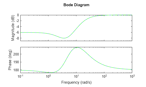

Create State-Space Model with Both Fixed and Tunable Parameters

This example shows how to create a state-space genss model having both fixed and tunable parameters.

$$A=\left[\begin{array}{cc}1& a+b\\ 0& ab\end{array}\right],B=\left[\begin{array}{c}-3.0\\ 1.5\end{array}\right],C=\left[\begin{array}{cc}0.3& 0\end{array}\right],D=0,$$

where a and b are tunable parameters, whose initial values are -1 and 3, respectively.

Create the tunable parameters using realp.

a = realp('a',-1);
b = realp('b',3);

Define a generalized matrix using algebraic expressions of a and b.

A = [1 a+b;0 a*b];

A is a generalized matrix whose Blocks property contains a and b. The initial value of A is [1 2;0 -3], from the initial values of a and b.

Create the fixed-value state-space matrices.

B = [-3.0;1.5];
C = [0.3 0];
D = 0;

Use ss to create the state-space model.

sys = ss(A,B,C,D)

Generalized continuous-time state-space model with 1 outputs, 1 inputs, 2 states, and the following blocks:
  a: Scalar parameter, 2 occurrences.
  b: Scalar parameter, 2 occurrences.

Type "ss(sys)" to see the current value and "sys.Blocks" to interact with the blocks.

sys is a generalized LTI model (genss) with tunable parameters a and b.

State-Space Model with Input and Output Delay

For this example, consider a SISO state-space model defined by the following state-space matrices:

$$A=\left[\begin{array}{cc}-1.5& -2\\ 1& 0\end{array}\right]B=\left[\begin{array}{c}0.5\\ 0\end{array}\right]C=\left[\begin{array}{cc}0& 1\end{array}\right]D=0$$

Considering an input delay of 0.5 seconds and an output delay of 2.5 seconds, create a state-space model object to represent the A, B, C and D matrices.

A = [-1.5,-2;1,0];
B = [0.5;0];
C = [0,1];
D = 0;
sys = ss(A,B,C,D,'InputDelay',0.5,'OutputDelay',2.5)

sys =
 
  A = 
         x1    x2
   x1  -1.5    -2
   x2     1     0
 
  B = 
        u1
   x1  0.5
   x2    0
 
  C = 
       x1  x2
   y1   0   1
 
  D = 
       u1
   y1   0
 
  Input delays (seconds): 0.5 
  Output delays (seconds): 2.5 
 
Continuous-time state-space model.

You can also use the get command to display all the properties of a MATLAB object.

get(sys)

                A: [2x2 double]
                B: [2x1 double]
                C: [0 1]
                D: 0
                E: []
           Scaled: 0
        StateName: {2x1 cell}
        StatePath: {2x1 cell}
        StateUnit: {2x1 cell}
    InternalDelay: [0x1 double]
       InputDelay: 0.5000
      OutputDelay: 2.5000
        InputName: {''}
        InputUnit: {''}
       InputGroup: [1x1 struct]
       OutputName: {''}
       OutputUnit: {''}
      OutputGroup: [1x1 struct]
            Notes: [0x1 string]
         UserData: []
             Name: ''
               Ts: 0
         TimeUnit: 'seconds'
     SamplingGrid: [1x1 struct]

For more information on specifying time delay for an LTI model, see Specifying Time Delays.

Stability Analysis of State-Space Systems

For this example, consider a state-space system object that represents the following state matrices:

$$A=\left[\begin{array}{ccc}-1.2& -1.6& 0\\ 1& 0& 0\\ 0& 1& 0\end{array}\right],B=\left[\begin{array}{c}1\\ 0\\ 0\end{array}\right],C=\left[\begin{array}{ccc}0& 0.5& 1.3\end{array}\right],D=0,$$

Create a state-space object sys using the ss command.

A = [-1.2,-1.6,0;1,0,0;0,1,0];
B = [1;0;0];
C = [0,0.5,1.3];
D = 0;
sys = ss(A,B,C,D);

Next, compute the closed-loop state-space model for a unit negative gain and find the poles of the closed-loop state-space system object sysFeedback.

sysFeedback = feedback(sys,1);
P = pole(sysFeedback)

P = 3×1 complex

  -0.2305 + 1.3062i
  -0.2305 - 1.3062i
  -0.7389 + 0.0000i

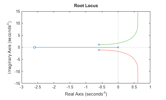
The feedback loop for unit gain is stable since all poles have negative real parts. Checking the closed-loop poles provides a binary assessment of stability. In practice, it is more useful to know how robust (or fragile) stability is. One indication of robustness is how much the loop gain can change before stability is lost. You can use the root locus plot to estimate the range of k values for which the loop is stable.

rlocus(sys)

Changes in the loop gain are only one aspect of robust stability. In general, imperfect plant modeling means that both gain and phase are not known exactly. Since modeling errors have the most detrimental effect near the gain crossover frequency (frequency where open-loop gain is 0dB), it also matters how much phase variation can be tolerated at this frequency.

You can display the gain and phase margins on a Bode plot as follows.

bode(sys)
grid

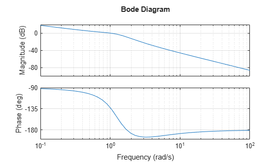
For a more detailed example, see Assessing Gain and Phase Margins.

Control Design using State-Space Models

For this example, design a 2-DOF PID controller with a target bandwidth of 0.75 rad/s for a system represented by the following matrices:

$$A=\left[\begin{array}{cc}-0.5& -0.1\\ 1& 0\end{array}\right],B=\left[\begin{array}{c}1\\ 0\end{array}\right],C=\left[\begin{array}{cc}0& 1\end{array}\right],D=0.$$

Create a state-space object sys using the ss command.

A = [-0.5,-0.1;1,0];
B = [1;0];
C = [0,1];
D = 0;
sys = ss(A,B,C,D)

sys =
 
  A = 
         x1    x2
   x1  -0.5  -0.1
   x2     1     0
 
  B = 
       u1
   x1   1
   x2   0
 
  C = 
       x1  x2
   y1   0   1
 
  D = 
       u1
   y1   0
 
Continuous-time state-space model.

Using the target bandwidth, use pidtune to generate a 2-DOF controller.

wc = 0.75;
C2 = pidtune(sys,'PID2',wc)

C2 =
 
                       1              
  u = Kp (b*r-y) + Ki --- (r-y) + Kd*s (c*r-y)
                       s              

  with Kp = 0.513, Ki = 0.0975, Kd = 0.577, b = 0.344, c = 0
 
Continuous-time 2-DOF PID controller in parallel form.

Using the type 'PID2' causes pidtune to generate a 2-DOF controller, represented as a pid2 object. The display confirms this result. The display also shows that pidtune tunes all controller coefficients, including the setpoint weights b and c, to balance performance and robustness.

For interactive PID tuning in the Live Editor, see the Tune PID Controller Live Editor task. This task lets you interactively design a PID controller and automatically generates MATLAB code for your live script.

For interactive PID tuning in a standalone app, use PID Tuner. See PID Controller Design for Fast Reference Tracking for an example of designing a controller using the app.

Connect Specific Inputs and Outputs of State-Space Models in a Feedback Loop

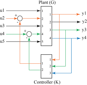
Consider a state-space plant G with five inputs and four outputs and a state-space feedback controller K with three inputs and two outputs. The outputs 1, 3, and 4 of the plant G must be connected the controller K inputs, and the controller outputs to inputs 4 and 2 of the plant.

For this example, consider two continuous-time state-space models for both G and K represented by the following set of matrices:

$$A_G=\left[\begin{array}{ccc}-3& 0.4& 0.3\\ -0.5& -2.8& -0.8\\ 0.2& 0.8& -3\end{array}\right],B_G=\left[\begin{array}{ccccc}0.4& 0& 0.3& 0.2& 0\\ -0.2& -1& 0.1& -0.9& -0.5\\ 0.6& 0.9& 0.5& 0.2& 0\end{array}\right],C_G=\left[\begin{array}{ccc}0& -0.1& -1\\ 0& -0.2& 1.6\\ -0.7& 1.5& 1.2\\ -1.4& -0.2& 0\end{array}\right],D_G=\left[\begin{array}{ccccc}0& 0& 0& 0& -1\\ 0& 0.4& -0.7& 0& 0.9\\ 0& 0.3& 0& 0& 0\\ 0.2& 0& 0& 0& 0\end{array}\right]$$

$$A_K=\left[\begin{array}{ccc}-0.2& 2.1& 0.7\\ -2.2& -0.1& -2.2\\ -0.4& 2.3& -0.2\end{array}\right],B_K=\left[\begin{array}{ccc}-0.1& -2.1& -0.3\\ -0.1& 0& 0.6\\ 1& 0& 0.8\end{array}\right],C_K=\left[\begin{array}{ccc}-1& 0& 0\\ -0.4& -0.2& 0.3\end{array}\right],D_K=\left[\begin{array}{ccc}0& 0& 0\\ 0& 0& -1.2\end{array}\right]$$

AG = [-3,0.4,0.3;-0.5,-2.8,-0.8;0.2,0.8,-3];
BG = [0.4,0,0.3,0.2,0;-0.2,-1,0.1,-0.9,-0.5;0.6,0.9,0.5,0.2,0];
CG = [0,-0.1,-1;0,-0.2,1.6;-0.7,1.5,1.2;-1.4,-0.2,0];
DG = [0,0,0,0,-1;0,0.4,-0.7,0,0.9;0,0.3,0,0,0;0.2,0,0,0,0];
sysG = ss(AG,BG,CG,DG)

sysG =
 
  A = 
         x1    x2    x3
   x1    -3   0.4   0.3
   x2  -0.5  -2.8  -0.8
   x3   0.2   0.8    -3
 
  B = 
         u1    u2    u3    u4    u5
   x1   0.4     0   0.3   0.2     0
   x2  -0.2    -1   0.1  -0.9  -0.5
   x3   0.6   0.9   0.5   0.2     0
 
  C = 
         x1    x2    x3
   y1     0  -0.1    -1
   y2     0  -0.2   1.6
   y3  -0.7   1.5   1.2
   y4  -1.4  -0.2     0
 
  D = 
         u1    u2    u3    u4    u5
   y1     0     0     0     0    -1
   y2     0   0.4  -0.7     0   0.9
   y3     0   0.3     0     0     0
   y4   0.2     0     0     0     0
 
Continuous-time state-space model.

AK = [-0.2,2.1,0.7;-2.2,-0.1,-2.2;-0.4,2.3,-0.2];
BK = [-0.1,-2.1,-0.3;-0.1,0,0.6;1,0,0.8];
CK = [-1,0,0;-0.4,-0.2,0.3];
DK = [0,0,0;0,0,-1.2];
sysK = ss(AK,BK,CK,DK)

sysK =
 
  A = 
         x1    x2    x3
   x1  -0.2   2.1   0.7
   x2  -2.2  -0.1  -2.2
   x3  -0.4   2.3  -0.2
 
  B = 
         u1    u2    u3
   x1  -0.1  -2.1  -0.3
   x2  -0.1     0   0.6
   x3     1     0   0.8
 
  C = 
         x1    x2    x3
   y1    -1     0     0
   y2  -0.4  -0.2   0.3
 
  D = 
         u1    u2    u3
   y1     0     0     0
   y2     0     0  -1.2
 
Continuous-time state-space model.

Define the feedout and feedin vectors based on the inputs and outputs to be connected in a feedback loop.

feedin = [4 2];
feedout = [1 3 4];
sys = feedback(sysG,sysK,feedin,feedout,-1)

sys =
 
  A = 
           x1      x2      x3      x4      x5      x6
   x1      -3     0.4     0.3     0.2       0       0
   x2    1.18   -2.56    -0.8    -1.3    -0.2     0.3
   x3  -1.312   0.584      -3    0.56    0.18   -0.27
   x4   2.948  -2.929   -2.42  -0.452   1.974   0.889
   x5   -0.84   -0.11     0.1    -2.2    -0.1    -2.2
   x6   -1.12   -0.26      -1    -0.4     2.3    -0.2
 
  B = 
            u1       u2       u3       u4       u5
   x1      0.4        0      0.3      0.2        0
   x2    -0.44       -1      0.1     -0.9     -0.5
   x3    0.816      0.9      0.5      0.2        0
   x4  -0.2112    -0.63        0        0      0.1
   x5     0.12        0        0        0      0.1
   x6     0.16        0        0        0       -1
 
  C = 
           x1      x2      x3      x4      x5      x6
   y1       0    -0.1      -1       0       0       0
   y2  -0.672  -0.296     1.6    0.16    0.08   -0.12
   y3  -1.204   1.428     1.2    0.12    0.06   -0.09
   y4    -1.4    -0.2       0       0       0       0
 
  D = 
          u1     u2     u3     u4     u5
   y1      0      0      0      0     -1
   y2  0.096    0.4   -0.7      0    0.9
   y3  0.072    0.3      0      0      0
   y4    0.2      0      0      0      0
 
Continuous-time state-space model.

size(sys)

State-space model with 4 outputs, 5 inputs, and 6 states.

sys is the resultant closed loop state-space model obtained by connecting the specified inputs and outputs of G and K.

Version History

Introduced before R2006a