Main Content

predict

Predict identified model K-step-ahead output

Description

This predict command computes the K-step-ahead output of an identified model using measured input-output data. To identify the model, you first collect all the input-output data and then estimate the model parameters offline. To perform online state estimation of a nonlinear system using real-time data, use the predict command for extended and unscented Kalman filters instead.

example

yp = predict(sys,data,K) predicts the output of an identified model sys, K steps ahead using the measured input-output data.

predict command predicts the output response over the time span of measured data. In contrast, forecast performs prediction into the future in a time range beyond the last instant of measured data. Use predict to validate sys over the time span of measured data.

data can be a timetable, a comma-separated input/output matrix pair, or an iddata object.

example

yp = predict(sys,data,K,opt) uses the option set opt to specify additional prediction options such as handling of initial conditions and data offsets.

example

[yp,ic,sys_pred] = predict(___) also returns the estimated values for initial conditions ic and a predictor model sys_pred. Use this syntax with any of the previous input argument combinations.

predict(sys,data,K,___) plots the predicted output. Use with any of the previous input argument combinations. To change display options in the plot, right-click the plot to access the context menu. For more details about the menu, see Tips.

You can also plot the predicted model response using the compare command. The compare command compares the prediction results with observed data and displays a quantitative goodness of fit.

predict(sys,Linespec,data,K,___) uses Linespec to specify the line type, marker symbol, and color.

predict(sys1,...,sysN,data,K,___) plots the predicted outputs for multiple identified models. predict automatically chooses colors and line styles.

example

predict(sys1,Linespec1,...,sysN,LinespecN,data,K,___) uses the line type, marker symbol, and color specified for each model.

Examples

collapse all

Simulate time-series data.

init_sys = idpoly([1 -0.99],[],[1 -1 0.2]);
opt = simOptions('AddNoise',true);
u = iddata([],zeros(400,0),1);
data = sim(init_sys,u,opt);

data is an iddata object containing the simulated response data of a time series model.

Estimate an ARMAX model by using data as estimation data.

na = 1;
nb = 2;
sys = armax(data(1:200),[na nb]);

Predict the output of the model using a prediction horizon of 4.

K = 4;
yp = predict(sys,data,K);

yp is an iddata object. The predicted output is returned in the OutputData property of the object.

Compare the predicted and estimated data outputs.

plot(data(201:400),yp(201:400));
legend('Estimation data','Predicted data');

Alternatively, to plot the predicted response and estimation data, use compare(sys,data,K).

Load the estimation data.

load sdata1 tt1;
data = tt1;

Estimate an ARX model of order [2 2 1].

sys1 = arx(data,[2 2 1]);

Estimate a transfer function with 2 poles.

 sys2 = tfest(data,2);

Create a predict option set to specify zero initial conditions for prediction.

opt = predictOptions('InitialCondition','z');

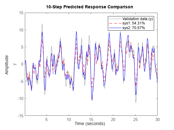
Plot the predicted outputs for the estimated models. Use the specified prediction option set, opt, and specify prediction horizon as 10. Specify line styles for plotting the predicted output of each system.

predict(sys1,'r--',sys2,'b',data,10,opt);

To change the display options, right-click the plot to access the context menu. For example, to view the estimation data, select Show Validation Data from the context menu. To view the prediction error, select Prediction Error Plot.

You can also plot the predicted response using the compare command. To do so, first create an option set for compare to specify the use of zero initial conditions.

opt = compareOptions('InitialCondition','z');
compare(data,sys1,'r--',sys2,'b',10,opt);

Use estimation data to estimate a model, and then compute the predicted model output and predictor model using the predict command. Simulate the predictor model to reproduce the predicted output.

Load estimation data.

load sdata3 umat3 ymat3 Ts

Estimate a polynomial model from the data.

sys = polyest(umat3,ymat3,[2 2 2 0 0 1]);

Predict the system response using prediction horizon 4.

K = 4;
[yp,ic,sysp] = predict(sys,umat3,ymat3,K);

yp is the predicted model response, ic contains the estimated initial conditions, and sysp is the predictor model.

Simulate the predictor model with inputs [data.OutputData,data.InputData] and initial conditions ic.

opt = simOptions;
opt.InitialCondition = ic;
ys = sim(sysp,[ymat3,umat3],opt);

Plot the predicted and simulated outputs.

ns = size(ys,1);
t = [1:Ts:ns]';

plot(t,yp,'b',t,ys,'.r');
legend('Predicted Output','Simulated Output')

Incorporate initial conditions that you obtained previously into your model prediction.

Load the data.

load iddata1ic z1i

Specify the ARMAX estimation option to estimate the initial state.

estimOpt = armaxOptions('InitialCondition','estimate');

Estimate an ARMAX model and return an initialCondition object ic that encapsulates the initial conditions in state-space form.

na = 2;
nb = 2;
nc = 2;
nk = 1;
[sys,ic] = armax(z1i,[na nb nc nk],estimOpt);

Specify the initial conditions for prediction.

predictOpt = predictOptions('InitialCondition',ic);

Predict the model and obtain the model response. Plot the response y with the measured data.

y = predict(sys,z1i,predictOpt);
plot(z1i,y)
legend('Measured Data','Predicted Response')

The measured and predicted responses show good agreement at the start of the prediction.

Perform model prediction using historical data to specify initial conditions. You first predict using the predict command and specify the historical data using the predictOptions option set. You then reproduce the predicted response by manually mapping the historical data to initial states.

Load a two-input, one-output dataset.

load iddata7 z7

Identify a fifth-order state-space model using the data.

sys = n4sid(z7,5);

Split the dataset into two parts.

zA = z7(1:15);
zB = z7(16:end);

Suppose that you want to compute the 10-step-ahead prediction of the response of the identified system for data zB. For initial conditions, use the signal values in zA as the historical record. That is, the input and output values for the time immediately preceding data in zB.

IO = struct('Input',zA.InputData,'Output',zA.OutputData);
opt = predictOptions('InitialCondition',IO);

Generate the 10-step-ahead prediction for data zB using the specified initial conditions and predict.

[yp,x0,Predictor] = predict(sys,zB,10,opt);

yp is the predicted model response, x0 are the initial states corresponding to the predictor model Predictor. You can simulate Predictor using x0 as initial conditions to reproduce yp.OutputData.

Now reproduce the output by manually mapping the historical data to initial states. To do so, minimize 1-step prediction errors over the time span of zA.

x0est = data2state(sys,zA);

x0est contains the values of the five states of sys at the time instant immediately after the most recent data sample in zA.

The Predictor has more states than the original system due to the 10-step prediction horizon. Specify the additional states induced by the horizon to zero initial values, and then append x0est.

x0Predictor = zeros(order(Predictor),1);
x0Predictor(end-4:end) = x0est;

Simulate the predictor using [zB.OutputData,zB.InputData] as the input signal and x0Predictor as initial conditions.

uData = [zB.OutputData,zB.InputData]; % signals required for prediction
[ysim,t,xsim] = lsim(Predictor,uData,[],x0Predictor);

Plot the predicted output of the predict command yp.OutputData and the manually computed results ysim.

plot(t,yp.OutputData,t,ysim, '.')

ysim is the same as yp.OutputData.

Input Arguments

collapse all

Identified model whose output is to be predicted, specified as one of the following:

If a model is unavailable, estimate sys from data using commands such as ar, armax, tfest, nlarx, and ssest.

Measured uniformly sampled input/output data, specified as a timetable, a comma-separated pair of numeric input/output matrices, or an iddata object. The specification for data depends on the data type.

Timetable

Specify data as a timetable that uses a regularly spaced time vector. containing variables that represent input and output channels.

Comma-Separated Matrix Pair

Specify data as a comma-separated pair of matrices that contain the input and output time-domain signal values u,y. Specify the input matrix with the dimensions Ns-by-Nu and the output matrix with the dimensions Ns-by-Ny, where Nu is the number of inputs, Ny is the number of outputs, and Ns is the number of samples.

For time-series data, specify [],y.

Use matrix-based data only for discrete-time models.

Data Object

Specify data as an iddata object that contains the input and output data. For time-series data (no inputs), specify data as an iddata object with no inputs.

For more information about working with estimation data types, see Data Domains and Data Types in System Identification Toolbox.

Prediction horizon, specified as one of the following:

  • Positive integer — Output yp is calculated K steps into the future, where K represents a multiple of data sample time.

    The output at time instant t is calculated using previously measured outputs up to time t-K and inputs up to the time instant t.

  • Inf — No previous outputs are used in the computation, and predict returns the same result as simulation using the sim command.

For Output-Error models, there is no difference between the K step-ahead predictions and the simulated output. This is because Output-Error models only use past inputs to predict future outputs.

Note

For careful model validation, a one-step-ahead prediction (K = 1) is usually not a good test for validating the model sys over the time span of measured data. Even the trivial one step-ahead predictor, y^(t)=y(t1),  can give good predictions. So a poor model may look fine for one-step-ahead prediction of data that has a small sample time. Prediction with K = Inf, which is the same as performing simulation with sim command, can lead to diverging outputs because low-frequency disturbances in the data are emphasized, especially for models with integration. Use a K value between 1 and Inf to capture the mid-frequency behavior of the measured data.

Prediction options, specified as a predictOptions option set. Use the option set to specify prediction options such as handling of initial conditions and data offsets.

Line style, marker, and color, specified as a character vector. For example, 'b' or 'b+:'.

For more information about configuring Linespec, see the Linespec argument of plot.

Output Arguments

collapse all

Predicted output response, returned in the same form as data.

When data is an iddata object, the OutputData property of yp stores the values of the predicted output. The time variable takes values in the range represented by data.SamplingInstants.

The output at time instant t is calculated using previously measured outputs up to time t-K and inputs up to the time instant t. In other words, the predicted response at time point r of measured data is stored in the r+K-1 sample of yp. Note that at time r, the future inputs u(r+1), u(r+2),..., u(r+K) required for prediction are assumed to be known. For multi-experiment data, yp contains a predicted data set for each experiment. The time span of the predicted outputs matches that of the observed data.

When sys is specified using an idnlhw or idnlgrey model, yp is the same as the simulated response computed using data.InputData as input.

Estimated initial conditions corresponding to the predictor model sys_pred, returned as a column vector, an initialCondition object, or a cell array.

  • If sys is a linear transfer function or polynomial model, then ic is an initialCondition object. The initialCondition object encapsulates the free response of sys, in state-space form, with the corresponding initial state vector.

  • If sys is any other type of linear or nonlinear dynamic model, then ic is an initial state vector, returned as a column vector of size equal to the number of states.

  • If data contains multiexperiment data, then ic is a cell array of size Ne, where Ne is the number of experiments.

To reproduce prediction results, you can simulate sys_pred using ic as the initial conditions. For an example, see Reproduce Prediction Results by Simulation.

If sys is an idnlarx model, ic is returned empty.

Predictor model, returned as a dynamic system model. For multi-experiment data, sys_pred is an array of models, with one entry for each experiment. You can use the predictor model sys_pred and estimated initial conditions ic to reproduce the results of prediction:

  • If sys is a linear model, the predictor model is returned as either a model of the same type as sys or as a state-space version of the model (idss). To reproduce the results of prediction, simulate sys_pred using [data.OutputData data.InputData] as the input and ic as the initial conditions. The simulation output is the same as the predicted output yp.OutputData. For an example, see Reproduce Prediction Results by Simulation.

  • When sys is a nonlinear grey-box model (idnlgrey) or Hammerstein-Wiener model (idnlhw), the noise-component of the model is trivial, and so the predictor model is the same as the model. sys_pred is returned empty. To reproduce the results of prediction, simulate sys using initial conditions ic. For a definition of the states of idnlhw models, see Definition of idnlhw States.

  • If sys is a nonlinear ARX model (idnlarx), sys_pred and ic are returned empty. You cannot reproduce the prediction results by simulation.

For discrete-time data that is time-domain or frequency-domain data with sample time Ts greater than zero, sys_pred is a discrete-time model, even if sys is a continuous-time model.

Tips

  • Right-clicking the plot of the predicted output opens the context menu, where you can access the following options:

    • Systems — Select systems to view predicted response. By default, the response of all systems is plotted.

    • Data Experiment — For multi-experiment data only. Toggle between data from different experiments.

    • Characteristics — View the following data characteristics:

      • Peak Value — View the absolute peak value of the data. Applicable for time–domain data only.

      • Peak Response — View peak response of the data. Applicable for frequency-response data only.

      • Mean Value — View mean value of the data. Applicable for time–domain data only.

    • Show — For frequency-domain and frequency-response data only.

      • Magnitude — View magnitude of frequency response of the system.

      • Phase — View phase of frequency response of the system.

    • Show Validation Data — Plot data used to predict the model response.

    • I/O Grouping — For datasets containing more than one input or output channel. Select grouping of input and output channels on the plot.

      • None — Plot input-output channels in their own separate axes.

      • All — Group all input channels together and all output channels together.

    • I/O Selector — For datasets containing more than one input or output channel. Select a subset of the input and output channels to plot. By default, all output channels are plotted.

    • Grid — Add grids to the plot.

    • Normalize — Normalize the y-scale of all data in the plot.

    • Full View — Return to full view. By default, the plot is scaled to full view.

    • Prediction Horizon — Set the prediction horizon, or choose simulation.

    • Initial Condition — Specify handling of initial conditions. Not applicable for frequency-response data.

      Specify as one of the following:

      • Estimate — Treat the initial conditions as estimation parameters.

      • Zero — Set all initial conditions to zero.

      • Absorb delays and estimate — Absorb nonzero delays into the model coefficients and treat the initial conditions as estimation parameters. Use this option for discrete-time models only.

    • Predicted Response Plot — Plot the predicted model response. By default, the response plot is shown.

    • Prediction Error Plot — Plot the error between the model response and prediction data.

    • Properties — Open the Property Editor dialog box to customize plot attributes.

Version History

Introduced before R2006a

expand all