Simulate and Predict Identified Model Output
You identify a model so that you can accurately compute a dynamic system response to an input. There are two ways of generating an identified model response:
Simulation computes the model response using input data and initial conditions.
Prediction computes the model response at some specified amount of time in the future using the current and past values of measured input and output values, as well as initial conditions.

In system identification, the goal is to create a realistic dynamic system model that can then be used or handed off for an application goal. In this context, the main roles of simulation and prediction within the System Identification Toolbox™ are to provide tools for model identification, and also for choosing, tuning, and validating these models.
You can:
Identify your model in a manner that minimizes either prediction (prediction focus) or simulation error (simulation focus)
Visualize your model response in comparison with other models and with data measurements
Validate your model by comparing its response with measured input/output data that was not used for the original model estimation
Your choice of simulation or prediction approach depends on what your application needs are, but also where you are in the system identification workflow:
When you are identifying your models, a one-step prediction focus generally produces the best results. This advantage is because, by using both input and output measurements, one-step prediction accounts for the nature of the disturbances. Accounting for disturbances provides the most statistically optimal results.
When you are validating your models, simulation usually provides the more perceptive approach for assessing how your model will perform under a wide range of conditions. Your application may drive prediction-based validation as well, however. For example, if you plan to use your model for control design, you can validate the model by predicting its response over a time horizon that represents the dominating time constants of the model.
You can work in either the time domain or the frequency domain, and remain consistent with the domain of the input/output data. For frequency-domain data, the simulation results are products of the Fourier transform of the input and frequency function of the model. Because frequency-response model identification ignores noise dynamics, simulation focus and one-step prediction focus yield the same identified model. For validation in the frequency domain, use simulation.
For examples, see:
What Are Simulation and Prediction?
You can get a more detailed understanding of the differences between simulation and prediction by applying these techniques to a simple first-order system.
Simulation
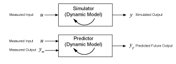
Simulation means computing the model response using input data and initial conditions. The time samples of the model response match the time samples of the input data used for simulation. In other words, given inputs u(t1, … ,tN), the simulation generates y(t1, … ,tN). The following diagram illustrates this flow.

For a continuous-time system, simulation means solving a differential equation. For a discrete-time system, simulation means directly applying the model equations.
For example, consider a dynamic model described by a first-order difference equation that uses a sample time of 1 second:
y(t+1) = ay(t) + bu(t),
where y is the output and u is the input.
This system is equivalent to the following block diagram.

Suppose that your model identification provides you with estimated parameter values of a = 0.9 and b = 1.5. Then the equation becomes:
y(t+1) = 0.9y(t) + 1.5u(t).
Now suppose that you want to compute the values y(1), y(2), y(3),... for given input values u(0) = 2, u(1) = 1, u(2) = 4,… Here, y(1) is the value of output at the first sampling instant. Using initial condition of y(0) = 0, the values of y(t) for times t = 1, 2, and 3 can be computed as:
y(1) = 0.9y(0) + 1.5u(0) =(0.9)(0) + (1.5)(2) = 3
y(2) = 0.9y(1) + 1.5u(1) =(0.9)(3) + (1.5)(1) = 4.2
y(3) = 0.9y(2) + 1.5u(2) =(0.9)(4.2) + (1.5)(4) = 9.78
Prediction
Prediction means projecting the model response k steps ahead into the future using the current and past values of measured input and output values. k is called the prediction horizon, and corresponds to predicting output at time kTs, where Ts is the sample time. In other words, given measured inputs um(t1, … ,tN+k) and measured outputs ym(t1, … ,tN) , the prediction generates yp(tN+k).
For example, suppose that you use sensors to measure the input signal um(t) and output signal ym(t) of the physical system described in the previous first-order equation. The equation becomes:
yp(t+1) = aym(t) + bum(t),
where y is the output and u is the input.
The predictor version of the previous simulation block diagram is:

At the 10th sampling instant (t = 10), the measured output ym(10) is 16 mm and the corresponding input um(10) is 12 N. Now, you want to predict the value of the output at the future time t = 11. Using the previous equation, the predicted output yp is:
yp(11) = 0.9ym(10) + 1.5um(10)
Hence, the predicted value of future output y(11) at time t = 10 is:
yp(11) = 0.9*16 + 1.5*12 = 32.4
In general, to predict the model response k steps into the future (k≥1) from the current time t, you must know the inputs up to time t+k and outputs up to time t:
yp(t+k)
=
f(um(t+k),um(t+k–1),...,um(t),um(t–1),...,um(0),
ym(t),ym(t–1),ym(t–2),...,ym(0))
um(0) and
ym(0) are the initial states.
f() represents the predictor,
which is a dynamic model whose form depends on the model structure.

The one-step-ahead predictor from the previous example, yp of the model y(t) + ay(t–1) = bu(t) is:
yp(t+1) = –ayp(t) + bum(t+1)
In this simple one-step predictor case, the newest prediction is based only on measurements. For multiple-step predictors, the dynamic model propagates states internally, using the previous predicted states in addition to the inputs. Each predicted output therefore arises from a combination of the measured input and outputs and the previous predicted outputs.
You can set k to any positive integer value up to the number of measured
data samples. If you set k to ∞, then no previous outputs are used in the
prediction computation, and prediction returns the same result as simulation. If you set
k to an integer greater than the number of data samples,
predict sets k to Inf and issues a
warning. If your intent is to perform a prediction in a time range beyond the last instant of
measured data, use forecast.
For an example showing prediction and simulation in MATLAB®, see Compare Predicted and Simulated Response of Identified Model to Measured Data.
Limitations on Prediction
Not all models support a predictive approach. For the previous dynamic model, , the structure supports use of past data. This support does not exist in
models of Output-Error (OE) structure (H(z) =
1). There is no information in past outputs that can be used for predicting
future output values. In these cases, prediction and simulation coincide. Even models that
generally do use past information can still have OE structure in special cases. State-space
models (idss) have OE structure when K=0. Polynomial
models (idpoly) also have OE structure, when a=c=d=1.
In these special cases, prediction and simulation are equivalent, and the disturbance model is
fixed to 1.
Compare Predicted and Simulated Response of Identified Model to Measured Data
This example shows how to visualize both the predicted model response and the simulated model response of an identified linear model.
Identify a third-order state-space model using the input/output measurements in z1.
load iddata1 z1;
sys = ssest(z1,3);
sys is a continuous-time identified state-space (idss) model. Here, sys is identified using the default 1-step prediction focus, which minimizes the 1-step prediction error. This focus generally provides the best overall model.
Now use compare to plot the predicted response. For this example, set the prediction horizon kstep to 10 steps, and use compare to plot the predicted response against the original measurement data. This setting of kstep specifies that each response point is 10 steps in the future with respect to the measurement data used to predict that point.
kstep = 10;
figure
compare(z1,sys,kstep)

In this plot, each data point represents the predicted output associated with output measurement data that was taken at least 10 steps earlier. For instance, the point at t=15 seconds is based on measurements taken at or prior to t=5 seconds.
The plot illustrates the differences between the model response and the original data. The percentage in the legend is the NRMSE fitness value. It represents how closely the predicted model output matches the data.
To improve your results, you can reduce the prediction horizon.
kstep = 5;
figure
compare(z1,sys,kstep)

The NRMSE fitness value has improved from the fitness value obtained in the 10-step case. In an actual application, there are various factors that influence how small the prediction horizon can be. These include time constants and application look-ahead requirements.
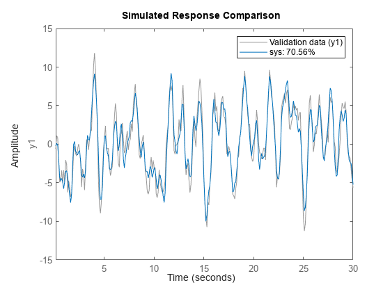
You can view the simulated response for comparison, rather than the predicted response, by using the kstep default for compare, which is Inf. With simulation, the response computation uses only the input data, not the measured output data.
figure
compare(z1,sys)

The simulated and the 10-step predicted responses yield similar overall fit percentages.
To change display options in the plot, right-click the plot to access the context menu. For example, to plot the error between the predicted output and measured output, select Error Plot from the context menu.
Compare Models Identified with Prediction and with Simulation Focus
This example shows how to identify models with prediction focus and with simulation focus. Compare the responses of prediction-focus and simulation-focus models against the original estimation data, and against validation data that was not used for estimation.
When you identify a model, the algorithm uses the 'Focus' option to determine whether to minimize prediction error or simulation error. The default is 'prediction'. You can change this by changing the 'Focus' option to 'simulation'.
Load the measurement data z1, and divide it into two halves z1e and z1v. One half is used for the model identification, and the other half for the model validation.
load iddata1 z1;
%z1e = z1(1:150); %To avoid ordqz stall
%z1v = z1(151:300);
z1e = z1(1:155);
z1v = z1(156:300);
Identify a third-order state-space model sys_pf using the input/output measurements in z1e. Use the default option 'Focus' option for this model, which is 'prediction'.
sys_pf = ssest(z1e,3);
sys_pf is a continuous-time identified state-space (idss) model.
Using the same set of measurement data, identify a second state-space model sys_sf which sets 'Focus' to 'simulation'.
opt = ssestOptions('Focus','simulation');
sys_sf = ssest(z1e,3,opt);
Use the compare function to simulate the response to both identified models.
figure
compare(z1e,sys_pf,sys_sf)

The model identified with predictive focus has a higher NRMSE fit value than the model identified with simulation focus.
Now perform a comparison against the validation data. This comparison shows how well the model performs with conditions that were not part of its identification.
figure
compare(z1v,sys_pf,sys_sf)

The fit values for both models improve. However, the model with prediction focus remains higher than the model with simulation focus.
See Also
forecast | predict | sim | compare