initialCondition

Initial condition representation for linear time-invariant systems

Since R2020b

Description

An initialCondition object encapsulates the initial-condition information for a linear time-invariant (LTI) model. The object generalizes the numeric vector representation of the initial states of a state-space model so that the information applies to linear models of any form—transfer functions, polynomial models, or state-space models.

You can estimate and retrieve initial conditions when you identify a linear model using commands such as tfest or compare model response to measured input/output data using compare. The software estimates the initial condition value by minimizing the simulation or prediction error against the measured output data. You can then apply those initial conditions in a subsequent simulation, using commands such as sim or predict, to confirm model performance with respect to the same measurement data. Use the initialCondition command to create an initialCondition object from a state-space model specification or from any LTI model of a free response.

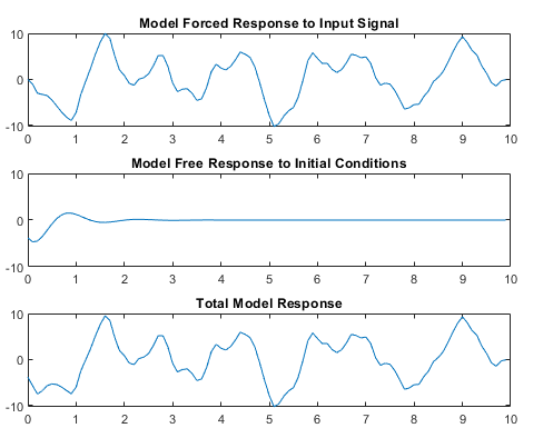
The initialCondition object can also be seen as a representation of the free response of a linear model. The simulation functions use this information to compute the model response in the following manner:

1. Compute the forced response of the model to the input signal. The forced response is the standard simulation output when there are no specified initial conditions.

2. Compute the impulse response of the model and scale the result to generate the free response of the model to the specified initial conditions.

3. Add the forced response and the free response together to form the total system response.

The figure illustrates this process.

For continuous systems (Ts = 0), the free response G(s) for the initial state vector x₀ is

$$G(s)=C{(sI-A)}^{-1}{x}_0$$

Here, C is equivalent to the state-space measurement matrix C and A is equivalent to the state-space state matrix A.

For discrete systems (Ts >0), the free response G(z) is

$$G(z)=zC{(zI-A)}^{-1}{x}_0$$

The initialCondition object represents the free response in state-space form. The object is a structure with properties containing the state-space A and C matrices and the initial state vector x₀. For idtf and idpoly models, using an initialCondition object is the only way to represent and use initial conditions for simulation. For idss models, you can use either an initialCondition object or a numeric initial state vector. When you obtain initial conditions ic for multiexperiment data, ic is an object array, with one initialCondition object for each experiment.

Creation

You can obtain an initialCondition object in one of four ways.

• Model estimation — Specify that the estimation function return the estimated initial condition that corresponds to the estimation input/output data. For example, you can use the following command to obtain the estimated initial condition ic for a transfer function model sys that is estimated with input/output data z.

  [sys,ic] = tfest(z,2,1)

  For an example, see Obtain Estimated Initial Conditions.

• Model-to-data comparison using any input/output data — Specify that compare return the estimated initial condition that the function estimates internally to support the fit assessment. For example, you can use the following command to obtain the initial condition ic for the linear model sys when determining the fit against input/output data z. yp is the simulated or predicted model output.

  [yp,fit,ic] = compare(z,sys)

  For an example, see Obtain Initial Conditions for New Data.

• Direct construction — Use the initialCondition command to encapsulate the state-space form of a free-response model in an initialCondition object.

  ic = initialCondition(A,X0,C,Ts)

  For an example, see Construct initialCondition Object from State-Space Model.

• Free-response model conversion — Use the initialCondition command to convert an LTI free-response model into an initialCondition object.

  ic = initialCondition(G)

  For an example, see Convert Free-Response Model to initialCondition Object.

For information on functions you can use to extract information from or transform initialCondition objects, see Object Functions.

Syntax

ic = initialCondition(A,X0,C,Ts)

ic = initialCondition(G)

Description

ic = initialCondition(A,X0,C,Ts) creates an initialCondition object that represents the free response to an initial condition, expressed in state-space form, of an LTI model.

$$\begin{array}{l}dx=Ax\\ y=Cx\\ x(0)=x_0\end{array}$$

ic stores this model in the form of properties. A and C correspond to a state-space realization of the model, X0 to the initial state vector x₀, and Ts to the sample time. You can use ic to specify initial conditions when simulating any type of LTI system.

ic = initialCondition(G) creates an initialCondition object corresponding to a linear model G of the free response.

Input Arguments

G — Free-response model

LTI model

Free-response model, specified as an LTI model with no inputs. In the continuous-time case, G must be strictly proper. In the discrete-time case, G must be biproper. For an example of using a free-response model to obtain an initialCondition object, see Convert Free-Response Model to initialCondition Object.

Properties

A — A matrix of state-space realization of LTI free response

numeric matrix

A matrix of the state-space realization of the LTI free response, specified as an N_x-by-N_x numeric matrix, where N_x is the number of states. For an example of using this property, see Obtain Estimated Initial Conditions.

X0 — Initial states of state-space realization of LTI free response

numeric vector

Initial states of the state-space realization of the LTI free response, specified as a numeric vector of length N_x. For an example of using this property, see Obtain Estimated Initial Conditions.

C — C matrix of state-space realization of LTI free response

numeric matrix

C matrix of the state-space realization of the LTI free response, specified as an N_y-by-N_x numeric matrix, where N_y is the number of outputs. For an example of using this property, see Obtain Estimated Initial Conditions.

Ts — Sample time

0 | –1 | positive scalar

Sample time of the LTI free response, specified as one of the following:

• Continuous-time model — 0

• Discrete-time model with a specified sampling time — Positive scalar representing the sampling period expressed in the unit specified by the TimeUnit property of the model

• Discrete-time model with unspecified sample time — –1

The sample time of an initialCondition object is the same as for the dynamic system model that the object corresponds to.

Object Functions

Functions applicable to initialCondition objects are those that can return, use, or convert the objects.

Initial Condition (IC) Role	LTI Function Type	Syntax Example	Example Links
Return estimated IC objects	All estimation functions, compare	[sys,ic] = tfest(data,2,1)	Obtain Estimated Initial Conditions Obtain Initial Conditions for Multiexperiment Data Obtain Initial Conditions for New Data
Use IC objects for model response	Option sets for model response functions	opt = simOptions('InitialCondition',ic)	Apply Initial Conditions in Simulation
Convert IC objects into Dynamic System Models (DSMs)	DSM object functions	g = idtf(ic)	Visualize Free Response to Initial Condition
Analyze models converted from IC objects	DSM analysis functions	y_g = impulse(g)	Visualize Free Response to Initial Condition

Estimate and Return Initial Conditions

tfest	Estimate transfer function model
procest	Estimate process model using time-domain or frequency-domain data
arx	Estimate parameters of ARX, ARIX, AR, or ARI model
armax	Estimate parameters of ARMAX, ARIMAX, ARMA, or ARIMA model using time-domain data
bj	Estimate Box-Jenkins polynomial model using time-domain data
oe	Estimate output-error polynomial model using time-domain or frequency-domain data
polyest	Estimate polynomial model using time- or frequency-domain data
compare	Compare identified model output with measured output

Use Initial Conditions

sim	Simulate response of identified model
simOptions	Option set for sim
predict	Predict state and state estimation error covariance at next time step using extended or unscented Kalman filter, or particle filter
predictOptions	Option set for predict
pe	Prediction error for identified model
peOptions	Option set for pe
resid	Compute and test residuals
residOptions	Option set for resid
compare	Compare identified model output with measured output
compareOptions	Option set for compare

Convert Initial Conditions to Dynamic System Model

idss	State-space model with identifiable parameters
idpoly	Polynomial model with identifiable parameters
idtf	Transfer function model with identifiable parameters

Analyze Free Model Response using idss Form

impulse	Impulse response plot of dynamic system; impulse response data
freqresp	Evaluate system response over a grid of frequencies

Examples

Obtain Estimated Initial Conditions

Estimate a transfer function model and obtain estimated initial conditions.

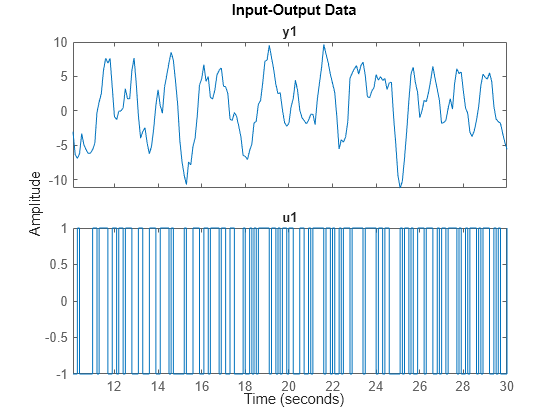
Load and plot the data.

load iddata1ic.mat z1i
plot(z1i)

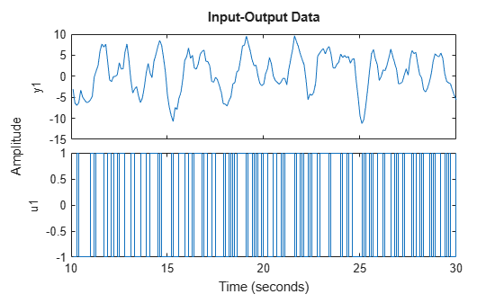
The output data does not start at 0.

Estimate a second-order transfer function sys_tf. Specify that the function return the initial conditions ic.

[sys_tf,ic] = tfest(z1i,2,1);

Examine the contents of ic. ic includes, in state-space form, the free response model defined by matrices A and C, the initial state vector X0, and the sample time Ts.

A = ic.A

A = 2×2

   -2.9841   -5.5848
    4.0000         0

C = ic.C

C = 1×2

    0.2957    5.2441

x0 = ic.X0

x0 = 2×1

   -0.9019
   -0.6161

Ts = ic.Ts

Ts = 0

ic is specific to the estimation data z1i. You can use ic to establish initial conditions when you simulate any LTI model using the input signal from z1i and compare the response with the z1i output signal.

Visualize Free Response to Initial Condition

Visualize the free response encapsulated in an initialCondition object by generating an impulse response.

Estimate a transfer function and return the initial condition ic_tf.

load iddata1ic z1i
[sys_tf,ic_tf] = tfest(z1i,2,1);
ic_tf

ic_tf = 
  initialCondition with properties:

     A: [2x2 double]
    X0: [2x1 double]
     C: [0.2957 5.2441]
    Ts: 0

ic_tf contains the information necessary to compute the free response to an initial condition.

Convert ic_tf into an idss object that can be passed to the impulse function.

ic_tfss = idss(ic_tf);

Create a time vector t that spans the data set. Compute the impulse response.

t = 0:0.1:9.9;
t = t';
yimp = impulse(ic_tfss,t);
plot(t,yimp)
title('Free Response to Initial Condition')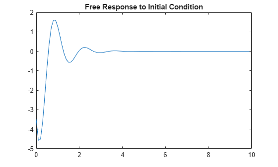

The free response is a transient that lasts for about four seconds.

Apply Initial Conditions in Simulation

Load the data and estimate a second-order transfer function sys. Return initial conditions in ic.

load iddata1ic z1i
[sys,ic] = tfest(z1i,2,1);

Simulate sys using the estimation data, but without incorporating the initial condition. Plot the simulated output with the measured output.

y_no_ic = sim(sys,z1i);
plot(y_no_ic,z1i)
legend('Model Response','Measured Output')

The measured and simulated outputs do not agree at the beginning of the simulation.

Incorporate ic into the simOptions option set opt. Simulate and plot the model response using opt.

opt = simOptions('InitialCondition',ic);
y_ic = sim(sys,z1i,opt);
plot(y_ic,z1i);
legend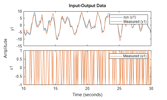('Model Response','Measured Output')

The simulation combines the model response to the input signal with the free response to the initial condition. The measured and simulated outputs now have better agreement at the beginning of the simulation.

Obtain Initial Conditions for New Data

An estimated initialCondition object is specific to the data from which you estimated it. If you want to simulate your model with new data, such as validation data, you need to estimate a new initial condition for that data. To do so, use the compare command.

Load data and split it into estimation and validation data sets.

load iddata1 z1
z1_est = z1(1:150);
z1_val = z1(151:300);
plot(z1_est,z1_val);
legend('Estimation Data','Validation Data')

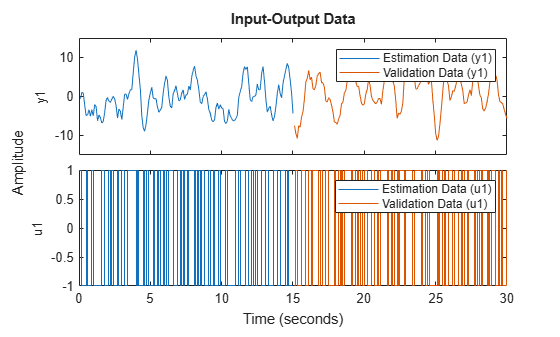
Examine the start points of each output data set.

e0 = z1_est.y(1)

e0 = -0.5872

v0 = z1_val.y(1)

v0 = -7.4390

The two data sets have different starting conditions.

Estimate a second-order transfer function model using z1_est. Return the estimated initial conditions in ic_est. Display the X0 property of ic_est. This property represents the estimated initial state vector that the free-response model defined by ic_est.A and ic_est.C responds to.

[sys,ic_est] = tfest(z1_est,2,1);
ic_est.X0

ans = 2×1

   -0.4082
    0.0095

You can use ic_est if you want to simulate sys using z1_est. Alternatively, you can use compare, which estimates the initial condition independently. Use compare twice, once to plot the data and once to return the results. Display the initial state vector ic_estc.X0 that compare estimates.

compare(z1_est,sys)

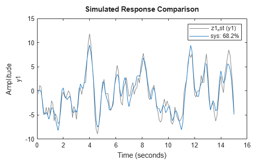
[yce,fit,ic_estc] = compare(z1_est,sys);
ic_estc.X0

ans = 2×1

   -0.4082
    0.0095

The initial state vector ic_estc.X0 is identical to ic_est.

Now evaluate the model with the validation data set. Estimate the initial conditions with the validation data.

compare(z1_val,sys)

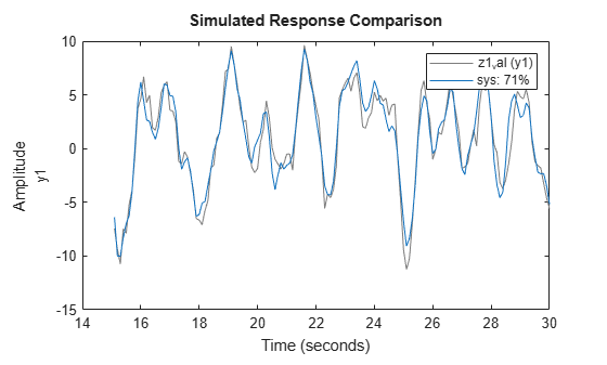
[ycv,fit,ic_valc] = compare(z1_val,sys);
ic_valc.X0

ans = 2×1

   -1.7536
   -0.9547

You can use ic_val when you simulate sys with the z1_val input signal and compare the model response to the z1_val output signal.

Obtain Initial Conditions for Multiexperiment Data

Estimate an initialCondition object array using multiexperiment data.

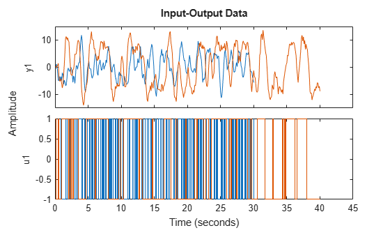
Load data from two experiments. Merge the two data sets into one multiexperiment data set.

load iddata1 z1
load iddata2 z2
z12 = merge(z1,z2)

z12 =
Time domain data set containing 2 experiments.

Experiment   Samples      Sample Time          
   Exp1         300            0.1             
   Exp2         400            0.1             
                                               
Outputs      Unit (if specified)               
   y1                                          
                                               
Inputs       Unit (if specified)               
   u1                                          
                                               

plot(z12)

Estimate the second-order transfer function sys and return the initial conditions in ic.

np = 2;
nz = 1;
[sys,ic] = tfest(z12,np,nz);
ic

ic=1×2 initialCondition array with properties:
    A
    X0
    C
    Ts

ic is an object array. Display the contents of each object.

ic(1,1)

ans = 
  initialCondition with properties:

     A: [2x2 double]
    X0: [2x1 double]
     C: [-0.7814 5.2530]
    Ts: 0

ic(1,2)

ans = 
  initialCondition with properties:

     A: [2x2 double]
    X0: [2x1 double]
     C: [-0.7814 5.2530]
    Ts: 0

Compare the A, X0, and C properties for each object.

A1 = ic(1,1).A

A1 = 2×2

   -3.4824   -5.5785
    4.0000         0

A2 = ic(1,2).A

A2 = 2×2

   -3.4824   -5.5785
    4.0000         0

C1 = ic(1,1).C

C1 = 1×2

   -0.7814    5.2530

C2 = ic(1,2).C

C2 = 1×2

   -0.7814    5.2530

X01 =ic(1,1).X0

X01 = 2×1

   -0.6528
   -0.0067

X02 =ic(1,2).X0

X02 = 2×1

    0.3076
   -0.0715

The A and C matrices are identical. These matrices represent the state-space form of sys. The X0 vectors are different. This difference results from the different initial conditions for the two experiments.

Construct initialCondition Object from State-Space Model

Estimate a state-space model and return the initial states. From the model and the initial state vector, construct an initialCondition object that can be used with any linear model.

Load and plot the data.

load iddata1ic z1i
plot(z1i)

Estimate a state-space model and obtain the estimated initial conditions.

First, set the 'InitialState' name-value pair argument in ssestOptions to 'estimate', which overrides the default setting of 'auto'. The 'estimate' setting always estimates the initial states. The 'auto' setting uses the 'zero' setting if the effect of the initial states on the overall model estimation error is relatively small, and can therefore result in an initial-state vector containing only zeros.

opt = ssestOptions;
opt = ssestOptions('InitialState','estimate');

Estimate a second-order state-space model sys_ss. Specify the output argument x0 to return the initial state vector. Specify the input argument opt to use your 'InitialState' setting. After estimating, examine x0.

[sys_ss,x0] = ssest(z1i,2,opt);
x0

x0 = 2×1

    0.0631
    0.0329

x0 is a nonzero initial state vector.

Simulate the model using x0 and compare the output with the original output data.

To use x0 as the initial condition, specify the 'InitialCondition' name-value pair argument in simOptions as x0.

opt = simOptions;
opt = simOptions('InitialCondition',x0);

Simulate the model using opt and store the response in xss.

xss = sim(sys_ss,z1i,opt);

Plot the model response with the original output data.

t = 0:0.1:19.9;
plot(t',[xss.y z1i.y])
legend('ss model','output data')
title('Simulated State-Space Model Using Estimated Initial States')

The simulation starts at a point close to the starting point of the data.

With the A and C matrices, x0, and the sample time Ts from sys_ss, construct an initialCondition object ic that you can use with a transfer function model.

A = sys_ss.A;
C = sys_ss.C;
Ts = sys_ss.Ts;
ic = initialCondition(A,x0,C,Ts)

ic = 
  initialCondition with properties:

     A: [2x2 double]
    X0: [2x1 double]
     C: [-61.3674 13.4811]
    Ts: 0

Estimate a transfer function model and simulate the model using ic as the initial condition. Store the response in xtf.

sys_tf = tfest(z1i,2,1);
opt = simOptions('InitialCondition',ic);
xtf = sim(sys_tf,z1i,opt);

Plot the model responses xss and xtf together.

plot(t',[xss.y xtf.y])
legend('ss model','tf model')
title('Simulated SS and TF Models with Equivalent Initial Conditions')

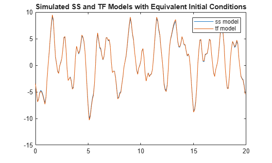
The models track each other closely throughout the simulation.

Convert Free-Response Model to initialCondition Object

Obtain the initial conditions when estimating a transfer function model. Convert the initialCondition into a free-response model, and the free-response model back into an initialCondition object.

Load the data and estimate a transfer function model sys. Obtain the estimated initial conditions ic.

load iddata1ic.mat z1i
[sys,ic] = tfest(z1i,2,1);

Convert ic into the idtf free-response model g.

g = idtf(ic);

Plot the impulse response of g.

impulse(g)
title('Impulse Response of g')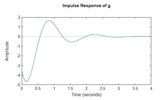

Convert g back into the initialCondition object ic1.

ic1 = initialCondition(g);

Plot the impulse response of ic1 by converting ic1 into an idss model.

impulse(idss(ic1))
title('Impulse Response of ic1 in idss form')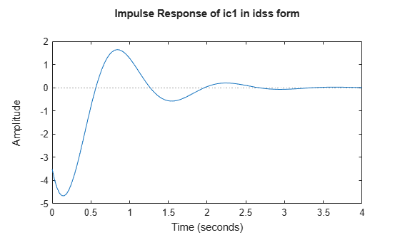

The impulse responses appear identical.

Compare ic and ic1.

ic.A

ans = 2×2

   -2.9841   -5.5848
    4.0000         0

ic1.A

ans = 2×2

   -2.9841   -5.5848
    4.0000         0

ic.X0

ans = 2×1

   -0.9019
   -0.6161

ic1.X0

ans = 2×1

     4
     0

ic.C

ans = 1×2

    0.2957    5.2441

ic1.C

ans = 1×2

   -0.8745   -1.7215

The A matrices of ic and ic1 are identical. The C matrix and the X0 vector are different. There are infinitely many state-space representations possible for a given linear model. The two objects are equivalent, as illustrated by the impulse responses.

Version History

Introduced in R2020b