Main Content

plot

Plot probability distribution object

Since R2022b

    Description

    example

    plot(pd) plots a probability density function (pdf) of the probability distribution object pd. If pd is created by fitting a probability distribution to the data, the pdf is superimposed over a histogram of the data.

    plot(ax,pd) plots into the axes specified by the Axes graphics object ax.

    example

    plot(___,Name=Value) specifies options using one or more name-value arguments in addition to any of the input argument combinations in the previous syntaxes. For example, you can indicate whether to plot a cumulative distribution function (cdf) or a probability plot instead of a pdf.

    H = plot(___) returns handles to the plotted graphics objects.

    Examples

    collapse all

    Generate random data points from a normal distribution with mean 0 and standard deviation 1.

    rng("default")  % Set the seed for reproducibility.

    Fit a normal distribution to the data.

    normaldata = normrnd(0,1,100,1);
    normalpd = fitdist(normaldata,"Normal")
    normalpd = 
      NormalDistribution
    
      Normal distribution
           mu = 0.123085   [-0.10756, 0.353731]
        sigma =   1.1624   [1.02059, 1.35033]


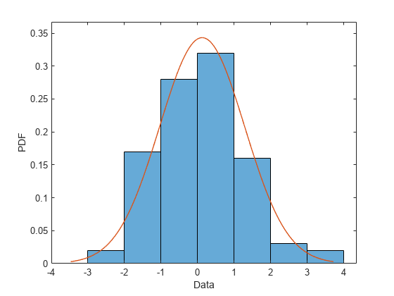
    normalpd is a NormalDistribution object that contains the parameter values for the normal distribution fit to the data, and the data. Plot a pdf for the normal distribution with a histogram of the data.

    plot(normalpd)

    Plot a cdf of the normal distribution fit to the data and a stairs plot of a cdf for the data.

    plot(normalpd,PlotType="cdf")

    Display a probability plot for the normal distribution fit to the data.

    plot(normalpd,PlotType="probability")

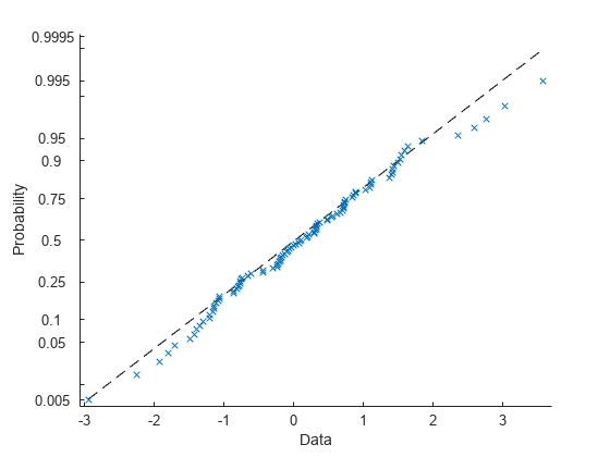
    The vertical axis is scaled so that the cdf for the fitted probability distribution is represented by a straight line.

    Create a multinomial distribution that has five outcomes with probabilities of 0.1, 0.2, 0.4, 0.2, and 0.1.

    multinomialpd = makedist("Multinomial",probabilities=[0.1 0.2 0.4 0.2 0.1])
    multinomialpd = 
      MultinomialDistribution
    
      Probabilities:
        0.1000    0.2000    0.4000    0.2000    0.1000


    Plot a pdf for the multinomial distribution.

    plot(multinomialpd)

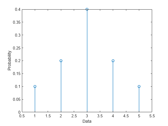
    The plot contains a Stem object that represents the probabilities for the data.

    Plot the pdf as a continuous distribution.

    plot(multinomialpd,Discrete=0)

    Plot the cdf of the fitted multinomial distribution as a stairs plot.

    plot(multinomialpd,PlotType="cdf")

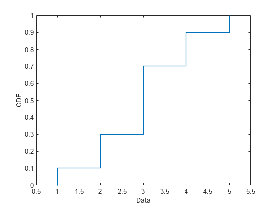
    Plot the cdf as a continuous distribution.

    plot(multinomialpd,PlotType="cdf",Discrete=0)
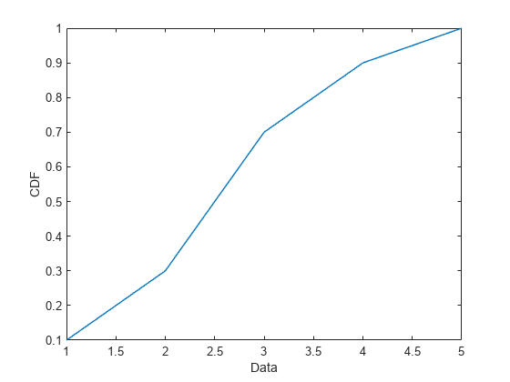
    Input Arguments

    collapse all

    Probability distribution, specified as one of the probability distribution objects in the following table.

    Distribution ObjectFunction or App Used to Create Probability Distribution Object
    BetaDistributionmakedist, fitdist, Distribution Fitter
    BinomialDistributionmakedist, fitdist, Distribution Fitter
    BirnbaumSaundersDistributionmakedist, fitdist, Distribution Fitter
    BurrDistributionmakedist, fitdist, Distribution Fitter
    ExponentialDistributionmakedist, fitdist, Distribution Fitter
    ExtremeValueDistributionmakedist, fitdist, Distribution Fitter
    GammaDistributionmakedist, fitdist, Distribution Fitter
    GeneralizedExtremeValueDistributionmakedist, fitdist, Distribution Fitter
    GeneralizedParetoDistributionmakedist, fitdist, Distribution Fitter
    HalfNormalDistributionmakedist, fitdist, Distribution Fitter
    InverseGaussianDistributionmakedist, fitdist, Distribution Fitter
    KernelDistributionfitdist, Distribution Fitter
    LogisticDistributionmakedist, fitdist, Distribution Fitter
    LoglogisticDistributionmakedist, fitdist, Distribution Fitter
    LognormalDistributionmakedist, fitdist, Distribution Fitter
    LoguniformDistributionmakedist
    MultinomialDistributionmakedist
    NakagamiDistributionmakedist, fitdist, Distribution Fitter
    NegativeBinomialDistributionmakedist, fitdist, Distribution Fitter
    NormalDistributionmakedist, fitdist, Distribution Fitter
    PiecewiseLinearDistributionmakedist
    PoissonDistributionmakedist, fitdist, Distribution Fitter
    RayleighDistributionmakedist, fitdist, Distribution Fitter
    RicianDistributionmakedist, fitdist, Distribution Fitter
    StableDistributionmakedist, fitdist, Distribution Fitter
    tLocationScaleDistributionmakedist, fitdist, Distribution Fitter
    TriangularDistributionmakedist
    UniformDistributionmakedist
    WeibullDistributionmakedist, fitdist, Distribution Fitter

    Axes for plot, specified as an Axes graphics object. If you do not specify the axes by using the ax input argument or the Parent name-value argument, the plot function plots into the current axes or creates an Axes object if one does not exist. For more information on creating an Axes graphics object, see axes and Axes Properties.

    Name-Value Arguments

    Specify optional pairs of arguments as Name1=Value1,...,NameN=ValueN, where Name is the argument name and Value is the corresponding value. Name-value arguments must appear after other arguments, but the order of the pairs does not matter.

    Example: Discrete=1,PlotType="cdf" plots a cumulative distribution function (cdf) of the probability distribution as a stairs plot.

    Plot type for the probability distribution, specified as one of the following.

    "pdf"Plot the probability density function (pdf). When pd is fit to data, the pdf is superimposed on a histogram of the data.
    "cdf"Plot the cumulative distribution function (cdf). When pd is fit to data, the cdf is superimposed over an empirical cdf.
    "probability"Display a probability plot using a cdf of the data and a cdf of the fitted probability distribution. This option is available only when pd is parametric and fit to data.

    Example: PlotType="probability"

    Data Types: char | string

    Indicator to plot as a discrete function, specified as 1 (true) or 0 (false). Specify Discrete=0 to display the pdf or cdf as a line plot. Specify Discrete=1 to display the pdf as a stem plot or to display the cdf as a stairs plot.

    The default value for Discrete is 1 when pd is a discrete probability distribution object and 0 when pd is a continuous probability distribution object. If pd is continuous, plot ignores the user-specified input for Discrete and plots continuous functions.

    Example: Discrete=0

    Data Types: logical

    Axes for plot, specified as an Axes graphics object. If you do not specify the axes by using the ax input argument or the Parent name-value argument, the plot function plots into the current axes or creates an Axes object if one does not exist. For more information on creating an Axes graphics object, see axes and Axes Properties.

    Output Arguments

    collapse all

    Handles to the plotted graphics objects, returned as a Line object, Stem object, Stairs object, or graphics array.

    • When PlotType is set to "pdf" or "cdf", and pd is not fit to data, H is a single handle corresponding to the pdf or cdf for the distribution.

    • When PlotType is set to "pdf" or "cdf", and pd is fit to data, H is a 1-by-2 graphics array. The first entry of the graphics array corresponds to the pdf or cdf for the distribution, and the second entry corresponds to the data.

    • When PlotType is set to "probability", H is a 2-by-1 graphics array with entries corresponding to the data and the distribution.

    The table below shows how the returned graphics object depends on whether the distribution is discrete, whether pd is fit to data, and the specified values for the name-value arguments Discrete and PlotType.

    Distribution TypeFit to DataDiscrete valuePlotType valueReturned Graphics Object
    DiscreteNo1"pdf"Stem
    "cdf"Stairs
    0"pdf"Line
    "cdf"Line
    Yes1"pdf"[Stem Patch]
    "cdf"[Stairs Stairs]
    "probability"[Line FunctionLine]
    0"pdf"[Line Patch]
    "cdf"[Line Stairs]
    "probability"[Line FunctionLine]
    ContinuousNo0"pdf"Line
    "cdf"Line
    Yes0"pdf"[Line Histogram]
    "cdf"[Line Stairs]
    "probability"[Line FunctionLine]

    Version History

    Introduced in R2022b