What is Model Predictive Control?

Model predictive control (MPC) is an optimal control technique in which the calculated control actions minimize a cost function for a constrained dynamical system over a finite, receding, horizon.

At each time step, an MPC controller receives or estimates the current state of the plant. It then calculates the sequence of control actions that minimizes the cost over the horizon by solving a constrained optimization problem that relies on an internal plant model and depends on the current system state. The controller then applies to the plant only the first computed control action, disregarding the following ones. In the following time step the process repeats.

The following picture shows the basic MPC control loop, with the controller receiving the measured outputs and disturbances from the plant, and using an internal prediction plant model to both estimate the state and to calculate a sequence of control moves that minimize a cost function over a given horizon. In general, minimizing the cost function involves reducing the error between the future plant outputs and a reference trajectory. The unmeasured disturbances only affect the plant.

MPC basic control loop

The lower part of the following picture shows in more detail the reference trajectory and the predicted plant outputs. The MPC controller uses its internal prediction model to predict the plant outputs over the prediction horizon p. The upper part of the picture shows the control moves planned by the MPC control as well as the first control move, which is the one actually applied to the plant. The control horizon is the number of planned moves, and might be smaller than the prediction horizon.

MPC signals and horizons

When the cost function is quadratic, the plant is linear and without constraints, and the horizon tends to infinity, MPC is equivalent to linear-quadratic Gaussian (LQG) control (or to a linear-quadratic regulator (LQR) control if the plant states are measured and no estimator is used).

In practice, despite the finite horizon, MPC often inherits many useful characteristics of traditional optimal control, such as the ability to naturally handle multi-input multi-output (MIMO) plants, the capability of dealing with time delays (possibly of different durations in different channels), and built-in robustness properties against modeling errors. Nominal stability can also be guaranteed by using specific terminal constraints. Other additional important MPC features are its ability to explicitly handle constraints and the possibility of making use of information on future reference and disturbance signals, when available.

For an introduction on the subject, see first two books in the bibliography sections. For an explanation of the controller internal model and its estimator, see MPC Prediction Models and Controller State Estimation, respectively. For an overview of the optimization problem, see Optimization Problem. For more information on the solvers, see QP Solvers.

Solving a constrained optimal control online at each time step can require substantial computational resources. However in some cases, such as for linear constrained plants, you can precompute and store the control law across the entire state space rather than solve the optimization in real time. This approach is known as explicit MPC.

MPC Design Workflow

In the simplest case (also known as traditional, or linear, MPC), in which both plant and constraints are linear and the cost function is quadratic, the general workflow to develop an MPC controller includes the following steps.

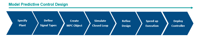
1. Specify plant — Define the internal plant model that the MPC controller uses to forecast plant behavior across the prediction horizon. Typically, you obtain this plant model by linearizing a nonlinear plant at a given operating point and specifying it as an LTI object, such as ss, tf, and zpk. You can also identify a plant using System Identification Toolbox™ software. Note that one limitation is that the plant cannot have a direct feedthrough between its control input and any output. For more information on this step, see Construct Linear Time Invariant Models, Specify Multi-Input Multi-Output Plants, Linearize Simulink Models, Linearize Simulink Models Using MPC Designer, and Identify Plant from Data.

2. Define signal types — For MPC design purposes, plant signals are usually categorized into different input and output types. You typically use setmpcsignals to specify, in the plant object defined in the previous step, whether each plant output is measured or unmeasured, and whether each plant input is a manipulated variable (that is, a control input) or a measured or unmeasured disturbance. Alternatively, you can specify signal types in MPC Designer. For more information, see MPC Signal Types.

3. Create MPC object — After specifying the signal types in the plant object, you create an mpc object in the MATLAB^® workspace (or in the MPC Designer), and specify, in the object, controller parameters such as the sample time, prediction and control horizons, cost function weights, constraints, and disturbance models. The following is an overview of the most important parameters that you need to select.

   1. Sample time — A typical starting guess consists of setting the controller sample time so that 10 to 20 samples cover the rise time of the plant.

   2. Prediction horizon — The number of future samples over which the controller tries to minimize the cost. It should be long enough to capture the transient response and cover the significant dynamics of the system. A longer horizon increases both performance and computational requirements. A typical prediction horizon is 10 to 20 samples.

   3. Control horizon — The number of free control moves that the controller uses to minimize the cost over the prediction horizon. Similarly to the prediction horizon, a longer control horizon increases both performance and computational requirements. A good rule of thumb for the control horizon is to set it from 10% to 20% of the prediction horizon while having a minimum of two to three steps. For more information on sample time and horizon, see Choose Sample Time and Horizons.

   4. Nominal Values — If your plant is derived from the linearization of a nonlinear model around an operating point, a good practice is to set the nominal values for input, state, state derivative (if nonzero), and output. Doing so allows you to specify constraints on the actual inputs and outputs (instead of doing so on the deviations from their nominal values), and allows you to simulate the closed loop and visualize signals more easily when using Simulink^® or the sim command.

   5. Scale factors — Good practice is to specify scale factors for each plant input and output, especially when their range and magnitude is very different. Appropriate scale factors improve the numerical condition of the underlying optimization problem and make weight tuning easier. A good recommendation is to set a scale factor approximatively equal to the span (the difference between the maximum and minimum value in engineering units) of the related signal. For more information, see Specify Scale Factors.

   6. Constraints — Constraints typically reflect physical limits. You can specify constraints as either hard (cannot be violated in the optimization) or soft (can be violated to a small extent). A good recommendation is to set hard constraints, if necessary, on the inputs or their rate of change, while setting output constraints, if necessary, as soft. Setting hard constraints on both input and outputs can lead to infeasibility and is in general not recommended. For more information, see Specify Constraints.

   7. Weights — You can prioritize the performance goals of your controller by adjusting the cost function tuning weights. Typically, larger output weights provide aggressive reference tracking performance, while larger weights on the manipulated variable rates promote smoother control moves that improve robustness. For more information, see Tune Weights.

   8. Disturbance and noise models — The internal prediction model that the controller uses to calculate the control action typically consists of the plant model augmented with models for disturbances and measurement noise affecting the plant. Disturbance models specify the dynamic characteristics of the unmeasured disturbances on the inputs and outputs, respectively, so they can be better rejected. By default, these disturbance models are assumed to be integrators (therefore allowing the controller to reject step-like disturbances) unless you specify them otherwise. Measurement noise is typically assumed to be white. For more information on plant and disturbance models see MPC Prediction Models, and Adjust Disturbance and Noise Models.

   After creating the mpc object, good practice is to use functions such as cloffset to calculate the closed loop steady state output sensitivities, therefore checking whether the controller can reject constant output disturbances. The more general review also inspects the object for potential problems. To perform a deeper sensitivity and robustness analysis for the time frames in which you expect no constraint to be active, you can also convert the unconstrained controller to an LTI system object using ss, zpk, or tf. For related examples, see Review Model Predictive Controller for Stability and Robustness Issues, Test MPC Controller Robustness Using MPC Designer, Compute Steady-State Output Sensitivity Gain, and Extract Controller.

   Note that many of the recommended parameter choices are incorporated in the default values of the mpc object; however, since each of these parameter is normally the result of several problem-dependent trade offs, you have to select the parameters that make sense for your particular plant and requirements.

4. Simulate closed loop — After you create an MPC controller, you typically evaluate the performance of your controller by simulating it in closed loop with your plant using one of the following options.

   • Using MATLAB, you can simulate the closed loop using sim (more convenient for linear plant models) or mpcmove (more flexible, allowing for more general discrete time plants or disturbance signals and for a custom state estimator).

   • Using Simulink, you can use the MPC Controller block (which takes your mpc object as a parameter) in closed loop with your plant model built in Simulink. This option allows for the greatest flexibility in simulating more complex systems and for easy generation of production code from your controller.

   • Using MPC Designer, you can simulate the linear closed loop response while at the same time tuning the controller parameters.

   Note that any of these options allows you to also simulate model mismatches (cases in which the actual plant is slightly different from the internal plant model that the controller uses for prediction). For a related example, see Simulating MPC Controller with Plant Model Mismatch. When reference and measured disturbances are known ahead of time, MPC can use this information (also known as look-ahead, or previewing) to improve the controller performance. See Signal Previewing for more information and Improving Control Performance with Look-Ahead (Previewing) for a related example. Similarly, you can specify tuning weights and constraints that vary over the prediction horizon. For related examples, see Update Constraints at Run Time, Vary Input and Output Bounds at Run Time, Tune Weights at Run Time, and Adjust Horizons at Run Time.

5. Refine design — After an initial evaluation of the closed loop you typically need to refine the design by adjusting the controller parameters and evaluating different simulation scenarios. In addition to the parameters described in step 3, you can consider:

   • Using manipulated variable blocking. For more information, see Manipulated Variable Blocking.

   • For over-actuated systems, setting reference targets for the manipulated variables. For a related example, see Setting Targets for Manipulated Variables.

   • Tuning the gains of the Kalman state estimator (or designing a custom state estimator). For more information and related examples, see Controller State Estimation, Custom State Estimation, and Implement Custom State Estimator Equivalent to Built-In Kalman Filter.

   • Specifying terminal constraints. For more information and a related example, see Terminal Weights and Constraints and Provide LQR Performance Using Terminal Penalty Weights.

   • Specifying custom constraints. For related examples, see Constraints on Linear Combinations of Inputs and Outputs and Use Custom Constraints in Blending Process.

   • Specifying off-diagonal cost function weights. For an example, see Specifying Alternative Cost Function with Off-Diagonal Weight Matrices.

6. Speed up execution — See MPC Controller Deployment.

7. Deploy controller — See MPC Controller Deployment.

Control Nonlinear and Time-Varying Plants

Often the plant to be controlled can be accurately approximated by a linear plant only locally, around a given operating point. This approximation might no longer be accurate as time passes and the plant operating point changes.

You can use several approaches to deal with these cases, from the simpler to more general and complicated.

1. Adaptive MPC — If the order (and the number of time delays) of the plant does not change, you can design a single MPC controller (for example for the initial operating point), and then at run-time you can update the controller prediction model at each time step (while the controller still assumes that the prediction model stays constant in the future, across its prediction horizon).

   Note that while this approach is the simplest, it requires you to continuously (that is, at each time step) calculate the linearized plant that has to be supplied to the controller. You can do so in three main ways.

   1. If you have a reliable plant model, you can extract the local linear plant online by linearizing the equations, assuming this process is not too computationally expensive. If you have simple symbolic equations for your plant model, you might be able to derive, offline, a symbolic expression of the linearized plant matrices at any given operating condition. Online, you can then calculate these matrices and supply them to the adaptive MPC controller without having to perform a numerical linearization at each time step. For an example using this strategy, see Adaptive MPC Control of Nonlinear Chemical Reactor Using Successive Linearization.

   2. Alternatively, you can extract an array of linearized plant models offline, covering the relevant regions of the state-input space, and then online you can use a linear parameter-varying (LPV) plant that obtains, by interpolation, the linear plant at the current operating point. For an example using this strategy, see Adaptive MPC Control of Nonlinear Chemical Reactor Using Linear Parameter-Varying System.

   3. If the plant is not accurately represented by a mathematical model, but you can assume a known structure with some estimates of its parameters, stability, and a minimal amount of input noise, you can use the past plant inputs and outputs to estimate a model of the plant online, although this can be somewhat computationally intensive. For an example using this strategy, see Adaptive MPC Control of Nonlinear Chemical Reactor Using Online Model Estimation.

   This approach requires an mpc object and either the mpcmoveAdaptive function or the Adaptive MPC Controller block. For more information, see Adaptive MPC and Model Updating Strategy.

2. Linear Time Varying MPC — This approach is a kind of adaptive MPC in which the controller knows in advance how its internal plant model changes in the future, and therefore uses this information when calculating the optimal control across the prediction horizon. Here, at every time step, you supply to the controller not only the current plant model but also the plant models for all the future steps, across the whole prediction horizon. To calculate the plant models for the future steps, you can use the manipulated variables and plant states predicted by the MPC controller at each step as operating points around which a nonlinear plant model can be linearized.

   This approach is particularly useful when the plant model changes considerably (but predictably) within the prediction horizon. It requires an mpc object and using mpcmoveAdaptive or the Adaptive MPC Controller block. For more information, see Time-Varying MPC.

3. Gain-Scheduled MPC — In this approach you design multiple MPC controllers offline, one for each relevant operating point. Then, online, you switch the active controller as the plant operating point changes. While switching the controller is computationally simple, this approach requires more online memory (and in general more design effort) than adaptive MPC. It should be reserved for cases in which the linearized plant models have different orders or time delays (and the switching variable changes slowly, with respect to the plant dynamics). To use gain-scheduled MPC. you create an array of mpc objects and then use the mpcmoveMultiple function or the Multiple MPC Controllers block for simulation. For more information, see Gain-Scheduled MPC. For an example, see Gain-Scheduled MPC Control of Nonlinear Chemical Reactor.

4. Nonlinear MPC — You can use this strategy to control highly nonlinear plants when all the previous approaches are unsuitable, or when you need to use nonlinear constraints or non-quadratic cost functions. This approach is more computationally intensive than the previous ones, and it also requires you to design an implement a nonlinear state estimator if the plant state is not completely available. Two nonlinear MPC approaches are available.

   1. Multistage Nonlinear MPC — For a multistage MPC controller, each future step in the horizon (stage) has its own decision variables and parameters, as well as its own nonlinear cost and constraints. Crucially, cost and constraint functions at a specific stage are functions only of the decision variables and parameters at that stage. While specifying multiple costs and constraint functions can require more design time, it also allows for an efficient formulation of the underlying optimization problem and a smaller data structure, which significantly reduces computation times compared to generic nonlinear MPC. Use this approach if your nonlinear MPC problem has cost and constraint functions that do not involve cross-stage terms, as is often the case. To use multistage nonlinear MPC you need to create an nlmpcMultistage object, and then use the nlmpcmove function or the Multistage Nonlinear MPC Controller block for simulation. For more information, see Multistage Nonlinear MPC.

   2. Generic Nonlinear MPC — This method is the most general, and computationally expensive, form of MPC. As it explicitly provides standard weights and linear bounds settings, it can be a good starting point for a design where the only nonlinearity comes from the plant model. Furthermore, you can use the RunAsLinearMPC option in the nlmpc object to evaluate whether linear, time varying, or adaptive MPC can achieve the same performance. If so, use these design options, and possibly evaluate gain scheduled MPC; otherwise, consider multistage nonlinear MPC. Use generic nonlinear MPC only as an initial design, or when all the previous design options are not viable. To use generic nonlinear MPC, you need to create an nlmpc object, and then use the nlmpcmove function or the Nonlinear MPC Controller block for simulation. For more information, see Generic Nonlinear MPC.

MPC Controller Deployment

When you are satisfied with the simulation performance of your controller design, you typically look for ways to speed up the execution, in an effort to both optimize the design for future simulations and to meet the stricter computational requirements of embedded applications.

You can use several strategies to improve the computational performance of MPC controllers.

1. Try to increase the sample time — The sampling frequency must be high enough to cover the significant bandwidth of the system. However, if the sample time is too small, not only do you reduce the available computation time for the controller but you must also use a larger prediction horizon to cover the system response, which increases computational requirements.

2. Try to shorten prediction and control horizons — Since both horizons directly impact the total number of decision variables and constraints in the resulting optimization problem, they heavily affect both memory usage and the number of required calculations. Therefore, check whether you can obtain similar tracking responses and robustness to uncertainties with shorter horizons. Note that sample time plays a role too. The sampling frequency needs to be high enough (equivalently the sample time small enough) to cover the significant bandwidth of the system. However, if the sample time is too small, not only you have a shorter available execution time on the hardware, but you also need a larger number of prediction steps to cover the system response, which results in a more computationally expensive optimization problem to be solved at each time step.

3. Use varying parameters only when needed — Normally Model Predictive Control Toolbox™ allows you to vary some parameters (such as weights or constraints coefficients) at run-rime. While this capability is useful in some cases, it considerably increases the complexity of the software. Therefore, unless specifically needed, for deployment, consider explicitly specifying such parameters as constants, thus preventing the possibility of changing them online. For related examples, see Update Constraints at Run Time, Vary Input and Output Bounds at Run Time, Tune Weights at Run Time, and Adjust Horizons at Run Time.

4. Limit the maximum number of iterations that your controller can use to solve the quadratic optimization problem, and configure it to use the current suboptimal solution when the maximum number of iterations is reached. Using a suboptimal solution shortens the time needed by the controller to calculate the control action, and in some cases it does not significantly decrease performance. In any case, since the number of iterations can change dramatically from one control interval to the next, for real time applications, it is recommended to limit the maximum number of iterations. Doing so helps ensuring that the worst-case execution time does not exceed the total computation time allowed on the hardware platform, which is determined by the controller sample time. For a related example, see Use Suboptimal Solution in Fast MPC Applications.

5. Tune the solver and its options — The default Model Predictive Control Toolbox solver is a "dense," "active set" solver based on the KWIK algorithm, and it typically performs well in many cases. However, if the total number of manipulated variables, outputs, and constraints across the whole horizon is large, you might consider using an interior point solver. For resource-constrained embedded applications, consider the ADMM solver. If the internal plant is highly open-loop unstable, consider using a sparse solver. For an overview of the optimization problem, see Optimization Problem. For more information on the solvers, see QP Solvers and Configure Optimization Solver for Nonlinear MPC. For related examples, see Simulate MPC Controller with a Custom QP Solver and Optimizing Tuberculosis Treatment Using Nonlinear MPC with a Custom Solver.

For application with extremely fast sample time, consider using explicit MPC. It can be proven that the solution to the linear MPC problem (quadratic cost function, linear plant and constraints) is piecewise affine (PWA) on polyhedra. In other words, the constraints divide the state space into polyhedral "critical" regions in which the optimal control action is an affine (linear plus a constant) function of the state. The idea behind explicit MPC is to precalculate, offline and once for all, these functions of the state for every region. These functions can then be stored in your controller. At run time, the controller then selects and applies the appropriate state feedback law, depending on the critical region that the current operating point is in. Since explicit MPC controllers do not solve an optimization problem online, they require much fewer computations and are therefore useful for applications requiring small sample times. On the other hand, they also have a much larger memory footprint. Indeed, excessive memory requirements can render this approach no longer viable for medium to large problems. Also, since explicit MPC pre-computes the controller offline, it does not support runtime updates of parameters such as weights, constraints or horizons.

To use explicit MPC, you need to generate an explicitMPC object from an existing mpc object and then use the mpcmoveExplicit function or the Explicit MPC Controller block for simulation. For more information, see Explicit MPC.

A final option to consider to improve computational performance of both implicit and explicit MPC is to simplify the problem. Some parameters, such as the number of constraints and the number state variables, greatly increase the complexity of the resulting optimization problem. Therefore, if the previous options are not satisfying, consider retuning these parameters (and potentially use a simpler lower-fidelity prediction model) to simplify the problem.

Once you are satisfied with the computational performance of your design, you can generate code for deployment to real-time applications from MATLAB or Simulink. For more information, see Generate Code and Deploy Controller to Real-Time Targets.