plotSlice
Plot of slices through fitted linear regression surface
Description
plotSlice( creates a figure
containing one or more plots, each representing a slice through the regression
surface predicted by mdl)mdl. Each plot shows the fitted response
values as a function of a single predictor variable, with the other predictor
variables held constant.
plotSlice also displays the 95% confidence bounds for the
response values. You can specify the type of confidence bounds, and select which
predictors to use for each slice plot. For more information, see Tips.
Examples
Load the carsmall sample data set.
load carsmallThe variables Weight and Model_Year contain data for the car weight and year of manufacture. The variable MPG contains data for miles per gallon.
Create a table from the data in Weight, Model_Year, and MPG by using the categorical and table functions. Fit a linear regression model of MPG as a function of Model_Year and Weight.
Model_Year = categorical(Model_Year);
tbl = table(MPG,Weight,Model_Year);
mdl = fitlm(tbl,"MPG ~ Model_Year + Weight^2");
mdl is a LinearModel object that contains the results of fitting a linear regression model to the data.
Create a slice plot for mdl.
plotSlice(mdl)

Each plot shows MPG as a function of a single predictor variable, Weight in the plot on the left and Model_Year in the plot on the right. The predictor is fixed at the value shown in the x-axis of each plot. The 95% confidence intervals for the continuous predictor Weight are represented by a blue shaded region. The 95% confidence intervals for the categorical predictor Model_Year are represented by error bars. The dashed lines indicate a selected point, and the table to the left of the plots shows the response value and confidence bounds for the selected point. You can select a different point by changing the predictor values in the x-axis labels or by dragging the dashed lines to a different location.
Change the value of Weight to 4000.
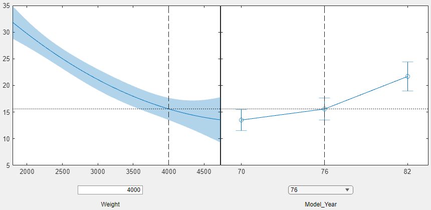
The right plot shows that MPG is smaller for cars with a weight of 4000, relative to cars with a weight of 3264, across all values for Model_Year.
Load the carsmall sample data set.
load carsmallThe variables Weight and Model_Year contain data for the car weight and year of manufacture. The variable MPG contains data for miles per gallon.
Create a table from the data in Weight, Model_Year, and MPG by using the categorical and table functions. Fit a linear regression model of MPG as a function of Model_Year and Weight.
Model_Year = categorical(Model_Year);
tbl = table(MPG,Weight,Model_Year);
mdl = fitlm(tbl,"MPG ~ Model_Year + Weight^2");
mdl is a LinearModel object that contains the results of fitting a linear regression model to the data.
Generate new predictor data for car weight and year of manufacture by using the linspace and ones functions.
Weight_New = linspace(2500,3500,100)';
Model_Year_New = categorical([ones(50,1).*70; ones(50,1).*76]);
Xnew = table(Weight_New,Model_Year_New,VariableNames=["Weight","Model_Year"]);
Create a slice plot for mdl using the new predictor data.
plotSlice(mdl,Xnew)

The left plot shows MPG as a function of Weight with Model_Year fixed at 76. The right plot shows MPG as a function of Model_Year with Weight fixed at 3000. The Confidence Interval Type options indicate that the confidence intervals are simultaneous and for the fitted responses. For more information, see Tips.
Load the census sample data set.
load censusThe variables pop and cdate contain data for the population size and the year the census was taken, respectively.
Fit a linear regression model using cdate as the predictor and pop as the response.
mdl = fitlm(cdate,pop);
mdl is a LinearModel object that contains the fitted linear regression model.
Create a slice plot for mdl.
plotSlice(mdl)

Because mdl has only one predictor, the slice plot displays a single set of axes containing a scatter plot of the training data. The regression line for mdl is shown in red together with a shaded region representing the 95% confidence intervals. The Confidence Interval Type options indicate that the confidence interval is simultaneous and for the fitted responses. For more information, see Tips.
Input Arguments
Tips
Use the Confidence Interval Type menu in the figure window to choose the type of confidence bounds. You can choose simultaneous or non-Simultaneous, and curve or observation.
Simultaneous or Non-Simultaneous
Simultaneous (default) —
plotSlicecomputes confidence bounds for the curve of the response values using Scheffé's method. The range between the upper and lower confidence bounds contains the curve consisting of true response values with 95% confidence.Non-Simultaneous —
plotSlicecomputes confidence bounds for the response value at each observation. The confidence interval for a response value at a specific predictor value contains the true response value with 95% confidence.
With simultaneous bounds, the entire curve of true response values is within the bounds at high confidence. By contrast, non-simultaneous bounds require only the response value at a single predictor value to be within the bounds at high confidence. Therefore, simultaneous bounds are wider than non-simultaneous bounds.
If you do not want the plot to display confidence bounds, you can clear the Show Confidence Intervals in Plot box.
Curve or Observation
A regression model for the predictor variables X and the response variable y has the form
y = f(X) + ε,
where f is a function of X and ε is a random noise term.
Curve (default) —
plotSlicepredicts confidence bounds for the fitted responses f(X).Observation —
plotSlicepredicts confidence bounds for the response observations y.
The bounds for y are wider than the bounds for f(X) because of the additional variability of the noise term.
Use the Predictors menu to select which predictors to use for each slice plot. If the regression model
mdlincludes more than eight predictors,plotSlicecreates plots for the first five predictors by default.
Alternative Functionality
Use
predictto return the predicted response values and confidence bounds. You can also specify the confidence level for confidence bounds by using the'Alpha'name-value pair argument of thepredictfunction. Note thatpredictfinds nonsimultaneous bounds by default whereasplotSlicefinds simultaneous bounds by default.A
LinearModelobject provides multiple plotting functions.When creating a model, use
plotAddedto understand the effect of adding or removing a predictor variable.When verifying a model, use
plotDiagnosticsto find questionable data and to understand the effect of each observation. Also, useplotResidualsto analyze the residuals of the model.After fitting a model, use
plotAdjustedResponse,plotPartialDependence, andplotEffectsto understand the effect of a particular predictor. UseplotInteractionto understand the interaction effect between two predictors. Also, useplotSliceto plot slices through the prediction surface.