predict

Predict responses of linear regression model

Syntax

ypred = predict(mdl,Xnew)

[ypred,yci] = predict(mdl,Xnew)

[ypred,yci] = predict(mdl,Xnew,Name,Value)

Description

ypred = predict(mdl,Xnew) returns the predicted response values of the linear regression model mdl to the points in Xnew.

[ypred,yci] = predict(mdl,Xnew) also returns confidence intervals for the responses at Xnew.

[ypred,yci] = predict(mdl,Xnew,Name,Value) specifies additional options using one or more name-value arguments. For example, you can specify the confidence level of the confidence interval and the prediction type.

Examples

Predict Response Values

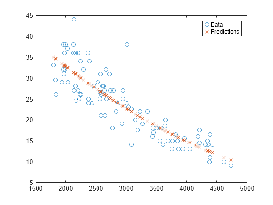
Create a quadratic model of car mileage as a function of weight from the carsmall data set.

load carsmall
X = Weight;
y = MPG;
mdl = fitlm(X,y,'quadratic');

Create predicted responses to the data.

ypred = predict(mdl,X);

Plot the original responses and the predicted responses to see how they differ.

plot(X,y,'o',X,ypred,'x')
legend('Data','Predictions')

Generate C/C++ Code for Prediction

Fit a linear regression model, and then save the model by using saveLearnerForCoder. Define an entry-point function that loads the model by using loadLearnerForCoder and calls the predict function of the fitted model. Then use codegen (MATLAB Coder) to generate C/C++ code. Note that generating C/C++ code requires MATLAB® Coder™.

This example briefly explains the code generation workflow for the prediction of linear regression models at the command line. For more details, see Code Generation for Prediction of Machine Learning Model at Command Line. You can also generate code using the MATLAB Coder app. For details, see Code Generation for Prediction of Machine Learning Model Using MATLAB Coder App.

Train Model

Load the carsmall data set, and then fit the quadratic regression model.

load carsmall
X = Weight;
y = MPG;
mdl = fitlm(X,y,'quadratic');

Save Model

Save the fitted quadratic model to the file QLMMdl.mat by using saveLearnerForCoder.

saveLearnerForCoder(mdl,'QLMMdl');

Define Entry-Point Function

Define an entry-point function named mypredictQLM that does the following:

• Accept measurements corresponding to X and optional, valid name-value pair arguments.

• Load the fitted quadratic model in QLMMdl.mat.

• Return predictions and confidence interval bounds.

function [yhat,ci] = mypredictQLM(x,varargin) %#codegen
%MYPREDICTQLM Predict response using linear model
%   MYPREDICTQLM predicts responses for the n observations in the n-by-1
%   vector x using the linear model stored in the MAT-file QLMMdl.mat, and
%   then returns the predictions in the n-by-1 vector yhat. MYPREDICTQLM
%   also returns confidence interval bounds for the predictions in the
%   n-by-2 vector ci.
CompactMdl = loadLearnerForCoder('QLMMdl');
[yhat,ci] = predict(CompactMdl,x,varargin{:});
end

Add the %#codegen compiler directive (or pragma) to the entry-point function after the function signature to indicate that you intend to generate code for the MATLAB algorithm. Adding this directive instructs the MATLAB Code Analyzer to help you diagnose and fix violations that would result in errors during code generation.

Note: If you click the button located in the upper-right section of this example and open the example in MATLAB®, then MATLAB opens the example folder. This folder includes the entry-point function file.

Generate Code

Generate code for the entry-point function using codegen (MATLAB Coder). Because C and C++ are statically typed languages, you must determine the properties of all variables in the entry-point function at compile time. To specify the data type and exact input array size, pass a MATLAB® expression that represents the set of values with a certain data type and array size. Use coder.Constant (MATLAB Coder) for the names of name-value pair arguments.

If the number of observations is unknown at compile time, you can also specify the input as variable-size by using coder.typeof (MATLAB Coder). For details, see Specify Variable-Size Arguments for Code Generation and Specify Types of Entry-Point Function Inputs (MATLAB Coder).

codegen mypredictQLM -args {X,coder.Constant('Alpha'),0.1,coder.Constant('Simultaneous'),true}

Code generation successful.

codegen generates the MEX function mypredictQLM_mex with a platform-dependent extension.

Verify Generated Code

Compare predictions and confidence intervals using predict and mypredictQLM_mex. Specify name-value pair arguments in the same order as in the -args argument in the call to codegen.

Xnew = sort(X);
[yhat1,ci1] = predict(mdl,Xnew,'Alpha',0.1,'Simultaneous',true);
[yhat2,ci2] = mypredictQLM_mex(Xnew,'Alpha',0.1,'Simultaneous',true);

The returned values from mypredictQLM_mex might include round-off differences compared to the values from predict. In this case, compare the values allowing a small tolerance.

find(abs(yhat1-yhat2) > 1e-6)

ans =

  0×1 empty double column vector

find(abs(ci1-ci2) > 1e-6)

ans =

  0×1 empty double column vector

The comparison confirms that the returned values are equal within the tolerance 1e–6.

Plot the returned values for comparison.

h1 = plot(X,y,'k.');
hold on
h2 = plot(Xnew,yhat1,'ro',Xnew,yhat2,'gx');
h3 = plot(Xnew,ci1,'r-','LineWidth',4);
h4 = plot(Xnew,ci2,'g--','LineWidth',2);
legend([h1; h2; h3(1); h4(1)], ...
    {'Data','predict estimates','MEX estimates','predict CIs','MEX CIs'});
xlabel('Weight');
ylabel('MPG');

Input Arguments

mdl — Linear regression model object

LinearModel object | CompactLinearModel object

Linear regression model object, specified as a LinearModel object created by using fitlm or stepwiselm, or a CompactLinearModel object created by using compact.

Xnew — New predictor input values

table | matrix

New predictor input values, specified as a table or matrix. Each row of Xnew corresponds to one observation, and each column corresponds to one variable.

• If Xnew is a table, it must contain predictors that have the same names as predictors in the PredictorNames property of mdl.

• If Xnew is a matrix, it must have the same number of variables (columns) in the same order as the predictor input used to create mdl. All variables used to create mdl must be numeric. To treat numerical predictors as categorical, specify the predictors using the CategoricalVars name-value argument when you create mdl.

Note that Xnew must also contain any predictor variables not used as predictors in the fitted model.

Data Types: single | double | table

Name-Value Arguments

Specify optional pairs of arguments as Name1=Value1,...,NameN=ValueN, where Name is the argument name and Value is the corresponding value. Name-value arguments must appear after other arguments, but the order of the pairs does not matter.

Example: [ypred,yci] = predict(Mdl,Xnew,'Alpha',0.01,'Simultaneous',true) returns the confidence interval yci with a 99% confidence level, computed simultaneously for all predictor values.

Alpha — Significance level

0.05 (default) | numeric value in the range [0,1]

Significance level for the confidence interval, specified as a numeric value in the range [0,1]. The confidence level of yci is equal to 100(1 – Alpha)%. Alpha is the probability that the confidence interval does not contain the true value.

Example: Alpha=0.01

Data Types: single | double

Prediction — Prediction type

"curve" (default) | "observation"

Prediction type, specified as "curve" or "observation".

A regression model for the predictor variables X and the response variable y has the form

y = f(X) + ε,

where f is a fitted regression function and ε is a random noise term.

• If Prediction is "curve", then the function predicts confidence bounds for f(Xnew), the fitted responses at Xnew.

• If Prediction is "observation", then the function predicts confidence bounds for y, the response observations at Xnew.

The bounds for y are wider than the bounds for f(X) because of the additional variability of the noise term.

Example: Prediction="observation"

Data Types: string | char

Simultaneous — Flag to compute simultaneous confidence bounds

false or 0 (default) | true or 1

Flag to compute simultaneous confidence bounds, specified as a numeric or logical 1 (true) or 0 (false).

• true — predict calculates confidence bounds for the curve of response values corresponding to all predictor values in Xnew, using Schefféʼs method. The range between the upper and lower bounds contains the curve that consists of true response values with 100(1 – α)% confidence.

• false — predict calculates confidence bounds for the response value at each observation in Xnew. The confidence interval for a response value at a specific predictor value contains the true response value with 100(1 – α)% confidence.

With simultaneous bounds, the entire curve of true response values is within the bounds at high confidence. By contrast, nonsimultaneous bounds require only the response value at a single predictor value to be within the bounds at high confidence. Therefore, simultaneous bounds are wider than nonsimultaneous bounds.

Example: Simultaneous=true

Output Arguments

ypred — Predicted response values

numeric vector

Predicted response values evaluated at Xnew, returned as a numeric vector.

yci — Confidence intervals for responses

two-column numeric matrix

Confidence intervals for the responses, returned as a two-column matrix in which each row provides one interval. The meaning of the confidence interval depends on the settings of the name-value arguments Alpha, Prediction, and Simultaneous.

Alternative Functionality

• feval returns the same predictions as predict. The feval function can take multiple input arguments, with one input for each predictor variable, which is simpler to use with a model created from a table or dataset array. Note that the feval function does not give confidence intervals on its predictions.

• random returns predictions with added noise.

• Use plotSlice to create a figure containing a series of plots, each representing a slice through the predicted regression surface. Each plot shows the fitted response values as a function of a single predictor variable, with the other predictor variables held constant.

Extended Capabilities

C/C++ Code Generation

Generate C and C++ code using MATLAB® Coder™.

Usage notes and limitations:

• Use saveLearnerForCoder, loadLearnerForCoder, and codegen (MATLAB Coder) to generate code for the predict function. Save a trained model by using saveLearnerForCoder. Define an entry-point function that loads the saved model by using loadLearnerForCoder and calls the predict function. Then use codegen to generate code for the entry-point function.

• To generate single-precision C/C++ code for predict, specify DataType="single" when you call the loadLearnerForCoder function.

• This table contains notes about the arguments of predict. Arguments not included in this table are fully supported.

  Argument	Notes and Limitations
  mdl	Suppose you train a linear model by using fitlm and specifying 'RobustOpts' as a structure with an anonymous function handle for the RobustWgtFun field, use saveLearnerForCoder to save the model, and then use loadLearnerForCoder to load the model. In this case, loadLearnerForCoder cannot restore the Robust property into the MATLAB® Workspace. However, loadLearnerForCoder can load the model at compile time within an entry-point function for code generation. For the usage notes and limitations of the model object, see Code Generation of the CompactLinearModel object.
  Xnew	Xnew must be a single-precision or double-precision matrix or a table containing numeric variables, categorical variables, or both. The number of rows, or observations, in Xnew can be a variable size, but the number of columns in Xnew must be fixed. If you want to specify Xnew as a table, then your model must be trained using a table, and you must ensure that your entry-point function for prediction: Accepts data as arrays Creates a table from the data input arguments and specifies the variable names in the table Passes the table to predict For an example of this table workflow, see Generate Code to Classify Data in Table. For more information on using tables in code generation, see Code Generation for Tables (MATLAB Coder) and Table Limitations for Code Generation (MATLAB Coder).
  Name-value pair arguments	Names in name-value arguments must be compile-time constants. For example, to allow a user-defined significance level in the generated code, include {coder.Constant('Alpha'),0} in the -args value of codegen (MATLAB Coder).

For more information, see Introduction to Code Generation.

GPU Arrays

Accelerate code by running on a graphics processing unit (GPU) using Parallel Computing Toolbox™.

This function fully supports GPU arrays. For more information, see Run MATLAB Functions on a GPU (Parallel Computing Toolbox).

Version History

Introduced in R2012a