fitPosterior
Fit posterior probabilities for support vector machine (SVM) classifier
Syntax
Description
ScoreSVMModel = fitPosterior(SVMModel)ScoreSVMModel containing the optimal
score-to-posterior-probability transformation function for two-class learning. For
more details, see Algorithms.
[
additionally returns the optimal score-to-posterior-probability transformation
function parameters.ScoreSVMModel,ScoreTransform]
= fitPosterior(SVMModel)
[
uses additional options specified by one or more name-value pair arguments. For
example, you can specify the number of folds or the holdout sample
proportion.ScoreSVMModel,ScoreTransform]
= fitPosterior(SVMModel,Name,Value)
Examples
Load the ionosphere data set. This data set has 34 predictors and 351 binary responses for radar returns, either bad ('b') or good ('g').
load ionosphereTrain a support vector machine (SVM) classifier. Standardize the data and specify that 'g' is the positive class.
SVMModel = fitcsvm(X,Y,'ClassNames',{'b','g'},'Standardize',true);
SVMModel is a ClassificationSVM classifier.
Fit the optimal score-to-posterior-probability transformation function.
rng(1); % For reproducibility
ScoreSVMModel = fitPosterior(SVMModel)
ScoreSVMModel =
ClassificationSVM
ResponseName: 'Y'
CategoricalPredictors: []
ClassNames: {'b' 'g'}
ScoreTransform: '@(S)sigmoid(S,-9.482430e-01,-1.217774e-01)'
NumObservations: 351
Alpha: [90×1 double]
Bias: -0.1342
KernelParameters: [1×1 struct]
Mu: [0.8917 0 0.6413 0.0444 0.6011 0.1159 0.5501 0.1194 0.5118 0.1813 0.4762 0.1550 0.4008 0.0934 0.3442 0.0711 0.3819 -0.0036 0.3594 -0.0240 0.3367 0.0083 0.3625 -0.0574 0.3961 -0.0712 0.5416 -0.0695 0.3784 … ] (1×34 double)
Sigma: [0.3112 0 0.4977 0.4414 0.5199 0.4608 0.4927 0.5207 0.5071 0.4839 0.5635 0.4948 0.6222 0.4949 0.6528 0.4584 0.6180 0.4968 0.6263 0.5191 0.6098 0.5182 0.6038 0.5275 0.5785 0.5085 0.5162 0.5500 0.5759 0.5080 … ] (1×34 double)
BoxConstraints: [351×1 double]
ConvergenceInfo: [1×1 struct]
IsSupportVector: [351×1 logical]
Solver: 'SMO'
Properties, Methods
Because the classes are inseparable, the score transformation function (ScoreSVMModel.ScoreTransform) is the sigmoid function.
Estimate scores and positive class posterior probabilities for the training data. Display the results for the first 10 observations.
[label,scores] = resubPredict(SVMModel);
[~,postProbs] = resubPredict(ScoreSVMModel);
table(Y(1:10),label(1:10),scores(1:10,2),postProbs(1:10,2),'VariableNames',...
    {'TrueLabel','PredictedLabel','Score','PosteriorProbability'})
ans=10×4 table
    TrueLabel    PredictedLabel     Score     PosteriorProbability
    _________    ______________    _______    ____________________

      {'g'}          {'g'}          1.4862           0.82216
      {'b'}          {'b'}         -1.0003           0.30433
      {'g'}          {'g'}          1.8685           0.86917
      {'b'}          {'b'}         -2.6457          0.084171
      {'g'}          {'g'}          1.2807           0.79186
      {'b'}          {'b'}         -1.4616           0.22025
      {'g'}          {'g'}          2.1674           0.89816
      {'b'}          {'b'}         -5.7085           0.00501
      {'g'}          {'g'}          2.4798           0.92224
      {'b'}          {'b'}         -2.7812          0.074781
Train a multiclass SVM classifier through the process of one-versus-all (OVA) classification, and then plot probability contours for each class. To implement OVA directly, see fitcecoc.
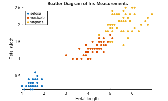
Load Fisher's iris data set. Use the petal lengths and widths as the predictor data.
load fisheriris
X = meas(:,3:4);
Y = species;
Examine a scatter plot of the data.
figure
gscatter(X(:,1),X(:,2),Y);
title('{\bf Scatter Diagram of Iris Measurements}');
xlabel('Petal length');
ylabel('Petal width');
legend('Location','Northwest');
axis tight
Train three binary SVM classifiers that separate each type of iris from the others. Assume that a radial basis function is an appropriate kernel for each, and allow the algorithm to choose a kernel scale. Define the class order.
classNames = {'setosa'; 'virginica'; 'versicolor'};
numClasses = size(classNames,1);
inds = cell(3,1); % Preallocation
SVMModel = cell(3,1);

rng(1); % For reproducibility
for j = 1:numClasses
    inds{j} = strcmp(Y,classNames{j});  % OVA classification
    SVMModel{j} = fitcsvm(X,inds{j},'ClassNames',[false true],...
        'Standardize',true,'KernelFunction','rbf','KernelScale','auto');
end
fitcsvm uses a heuristic procedure that involves subsampling to compute the value of the kernel scale.
Fit the optimal score-to-posterior-probability transformation function for each classifier.
for j = 1:numClasses
    SVMModel{j} = fitPosterior(SVMModel{j});
end
Warning: Classes are perfectly separated. The optimal score-to-posterior transformation is a step function.
Define a grid to plot the posterior probability contours. Estimate the posterior probabilities over the grid for each classifier.
d = 0.02;
[x1Grid,x2Grid] = meshgrid(min(X(:,1)):d:max(X(:,1)),...
    min(X(:,2)):d:max(X(:,2)));
xGrid = [x1Grid(:),x2Grid(:)];

posterior = cell(3,1);
for j = 1:numClasses
    [~,posterior{j}] = predict(SVMModel{j},xGrid);
end
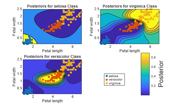
For each SVM classifier, plot the posterior probability contour under the scatter plot of the data.
figure
h = zeros(numClasses + 1,1); % Preallocation for graphics handles
for j = 1:numClasses
subplot(2,2,j)
contourf(x1Grid,x2Grid,reshape(posterior{j}(:,2),size(x1Grid,1),size(x1Grid,2)));
hold on
h(1:numClasses) = gscatter(X(:,1),X(:,2),Y);
title(sprintf('Posteriors for %s Class',classNames{j}));
xlabel('Petal length');
ylabel('Petal width');
legend off
axis tight
hold off
end
h(numClasses + 1) = colorbar('Location','EastOutside',...
    'Position',[[0.8,0.1,0.05,0.4]]);
set(get(h(numClasses + 1),'YLabel'),'String','Posterior','FontSize',16);
legend(h(1:numClasses),'Location',[0.6,0.2,0.1,0.1]);
Estimate the score-to-posterior-probability transformation function after training an SVM classifier. Use cross-validation during the estimation to reduce bias, and compare the run times for 10-fold cross-validation and holdout cross-validation.
Load the ionosphere data set.
load ionosphereTrain an SVM classifier. Standardize the data and specify that 'g' is the positive class.
SVMModel = fitcsvm(X,Y,'ClassNames',{'b','g'},'Standardize',true);
SVMModel is a ClassificationSVM classifier.
Fit the optimal score-to-posterior-probability transformation function. Compare the run times from using 10-fold cross-validation (the default) and a 10% holdout test sample.
rng(1); % For reproducibility
tic;    % Start the stopwatch
SVMModel_10FCV = fitPosterior(SVMModel);
toc     % Stop the stopwatch and display the run time
Elapsed time is 0.827798 seconds.
tic;
SVMModel_HO = fitPosterior(SVMModel,'Holdout',0.10);
toc
Elapsed time is 0.160244 seconds.
Although both run times are short because the data set is relatively small, SVMModel_HO fits the score transformation function much faster than SVMModel_10FCV. You can specify holdout cross-validation (instead of the default 10-fold cross validation) to reduce run time for larger data sets.
Input Arguments
Name-Value Arguments
Output Arguments
More About
Tips
This process describes one way to predict positive class posterior probabilities.
Train an SVM classifier by passing the data to
fitcsvm. The result is a trained SVM classifier, such asSVMModel, that stores the data. The software sets the score transformation function property (SVMModel.ScoreTransformation) tonone.Pass the trained SVM classifier
SVMModeltofitSVMPosteriororfitPosterior. The result, such as,ScoreSVMModel, is the same trained SVM classifier asSVMModel, except the software setsScoreSVMModel.ScoreTransformationto the optimal score transformation function.Pass the predictor data matrix and the trained SVM classifier containing the optimal score transformation function (
ScoreSVMModel) topredict. The second column in the second output argument ofpredictstores the positive class posterior probabilities corresponding to each row of the predictor data matrix.If you skip step 2, then
predictreturns the positive class score rather than the positive class posterior probability.
After fitting posterior probabilities, you can generate C/C++ code that predicts labels for new data. Generating C/C++ code requires MATLAB® Coder™. For details, see Introduction to Code Generation for Statistics and Machine Learning Functions.
Algorithms
The software fits the appropriate score-to-posterior-probability transformation
function by using the SVM classifier SVMModel and by conducting
10-fold cross-validation using the stored predictor data (SVMModel.X)
and the class labels (SVMModel.Y), as outlined in [1]. The transformation function computes the posterior probability that an observation
is classified into the positive class (SVMModel.Classnames(2)).
If the classes are inseparable, then the transformation function is the sigmoid function.
If the classes are perfectly separable, then the transformation function is the step function.
In two-class learning, if one of the two classes has a relative frequency of 0, then the transformation function is the constant function. The
fitPosteriorfunction is not appropriate for one-class learning.The software stores the optimal score-to-posterior-probability transformation function in
ScoreSVMModel.ScoreTransform.
If you re-estimate the score-to-posterior-probability
transformation function, that is, if you pass an SVM classifier to
fitPosterior or fitSVMPosterior and its
ScoreTransform property is not none, then the software:
Displays a warning
Resets the original transformation function to
'none'before estimating the new one
Alternative Functionality
You can also fit the posterior probability function by using fitSVMPosterior. This function is similar to
fitPosterior, except it is more broad because it accepts a wider
range of SVM classifier types.
References
[1] Platt, J. “Probabilistic outputs for support vector machines and comparisons to regularized likelihood methods.” Advances in Large Margin Classifiers. Cambridge, MA: The MIT Press, 2000, pp. 61–74.
Extended Capabilities
Version History
Introduced in R2014a