Frequency Response Estimator
Estimate plant frequency responses during simulation or in real time
Libraries:
Simulink Control Design /
Frequency Response Estimation
Description
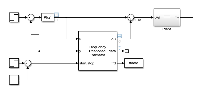
Use the Frequency Response Estimator block to perform experiment-based estimation in real time with a physical plant or in a Simulink® model during simulation. To obtain an estimated frequency response, the block simultaneously:
Injects perturbation signals into the plant at the nominal operating point
Collects response data from the plant output
Computes the estimated frequency response
You specify the frequencies at which to perturb the plant and measure system response. You trigger the estimation process via a start/stop signal. This signal lets you start estimation at any time, typically when the plant is at the nominal operating point. You stop the estimation after the frequency responses converge.
You can use online frequency response estimation with any stable SISO plant. For an unstable plant, online estimation works in a closed-loop configuration, provided that the closed loop is internally stable. A closed-loop system is internally stable if and only if the roots of the nominal closed-loop characteristic equation all lie in the open left half-plane. For a plant with transfer function G = NG/DG and controller C = NC/DC, the characteristic equation is:
DGDC + NGNC = 0.
In practice, this condition means that no unstable poles in G are stabilized by pole-zero cancellation in GC. Do not use online estimation with an unstable plant that does not meet this condition.
You can generate code and deploy the Frequency Response Estimator block on hardware to perform the estimation in real time. The block supports code generation with Simulink Coder™, Embedded Coder®, and Simulink PLC Coder™. It does not support code generation with HDL Coder™.
For more information about using the Frequency Response Estimator block, see:
For more general information about online frequency response estimation, see Online Frequency Response Estimation Basics.
Examples
Online Frequency Response Estimation During Simulation
Perform online frequency response estimation during model simulation using the Frequency Response Estimator block.
Collect Frequency Response Experiment Data for Offline Estimation
Use the Frequency Response Estimator block to perform a frequency response estimation experiment and store the data for later estimation offline.
Online Estimation of Frequency Responses of a Nonlinear Plant
Use the Frequency Response Estimator block to perform online estimation of a nonlinear plant at different nominal operating points.
Ports
Input
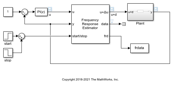
Insert the block into your system such that this port accepts a control signal or other plant input signal. For instance, in a closed-loop configuration, you can connect this port as shown in the following diagram.
In an open-loop configuration, you can connect this input port to a source that drives your plant to the desired operating point for estimation. For instance, you can use a Constant block set to an appropriate value.
Data Types: single | double
Connect this port to the plant output.
Data Types: single | double
To start and stop the estimation process, provide a signal at the
start/stop port. When the value of the signal changes
from:
Negative or zero to positive, the experiment starts
Positive to negative or zero, the experiment stops
Typically, you can use a signal that changes from 0 to 1 to start the experiment, and from 1 to 0 to stop it. When the experiment is not running, the block adds no perturbation at the u + Δu or Δu port. In this state, the block has no impact on plant behavior.
Start the experiment when the plant is at the desired equilibrium operating point. In a closed-loop configuration, use the controller to drive the plant to the operating point. In an open-loop configuration, you can use a source block connected to u to drive the plant to the operating point.
Let the experiment run long enough for the algorithm to collect sufficient data for a good estimate at all frequencies it probes. The block displays a recommended experiment length in the Experiment Length section of the block parameters. This value is based on the experiment mode and the frequencies you specify for the experiment.
When Experiment mode is Sinestream, the recommended experiment length is:
where:
ωi is the ith frequency specified in the Frequencies parameter (in rad/s).
Nfreq is the number of frequencies in Frequencies.
Nset,i is the corresponding value of the Number of settling periods parameter.
Nestim,i is the corresponding value of the Number of estimation periods parameter.
Ts is the experiment sampling time, specified by the Sample time (Ts) parameter.
When Experiment mode is Superposition, the recommended experiment length is six times the longest period. If your system does not require much time for the decay of transients or for the averaging away of noise, then you can use a shorter experiment length. For more information about how to determine experiment length in superposition mode, see Experiment Length and Data-Collection Window in Superposition Mode.
When Experiment mode is PRBS (since R2023a), the recommended experiment length is:
where:
Ts is the experiment sampling time, specified by the Sample time (Ts) parameter.
n is the PRBS signal order, specified by the Signal order parameter.
Np is the number of periods in the PRBS signal, specified by the Number of periods parameter.
Avoid any load disturbance to the plant during the experiment. Load disturbance can distort the plant output and reduce the accuracy of the frequency-response estimation.
Data Types: single | double
Supply a value for the Frequencies parameter. See that parameter for information about how to choose frequencies.
When you supply frequencies via this port, specify the number of frequencies with the Number of frequencies in the excitation signal parameter.
Dependencies
To enable this port, in Excitation Signal Source, select External ports.
Data Types: single | double
Supply a value for the Amplitudes parameter. See that parameter for details.
Dependencies
To enable this port, in Excitation Signal Source, select External Ports.
Data Types: single | double
Output
Insert the block into your system such that this port feeds the input signal to your plant, such as in the following diagram.
When the experiment is running (start/stop positive), the block injects test signals into the plant at this port. If you have any saturation or rate limit protecting the plant, feed the signal from u + Δu into it.
When the experiment is not running (start/stop zero or negative), the block passes signals unchanged from u to u + Δu. In this state, the block has no effect on the plant.
Dependencies
To enable this port, in Output Signal Configuration, select control action + perturbation.
Data Types: single | double
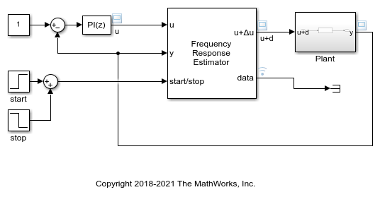
The block generates a perturbation signal at this port. Typically, you inject the perturbation from this port via a sum block, as shown in the following diagram.
When the experiment is running (start/stop positive), the block generates perturbation signals at this port.
When the experiment is not running (start/stop zero or negative), the signal at this port is zero. In this state, the block has no effect on the plant.
Dependencies
To enable this port, in Output Signal Configuration, select perturbation only.
Data Types: single | double
The signal at this port contains the data that the block collects during the frequency-response estimation experiment, including the perturbation signal applied to the plant and the measured plant response. Use this port when you want to log experiment data for later use. For instance, you can conserve resources in a deployed environment by logging the data and performing the estimation offline (see Estimation Mode). There are two ways to access the frequency response experiment data.
Use a To Workspace block to write the data to the MATLAB® workspace as a structure containing timeseries data. The Save format parameter of the To Workspace block must be
Timeseries. The structure has the following fields:Ready— Logical signal indicating which time steps are included in the estimation computation (1) and which are excluded (0). For instance, for sinestream mode, this signal is 1 only for data that falls within the periods determined by the Number of settling periods and Number of estimation periods parameters. In superposition mode, the signal is 1 only for data that falls within the window described in Experiment Length and Data-Collection Window in Superposition Mode. For PRBS signals, this is 1 only for data that falls within the actual experiment length.Perturbation— Sinusoidal perturbationsΔuapplied to the plantPlantInput— Plant input signalu + Δu, whereuis the signal collected at the block input port yPlantOutput— Plant output signal collected at block input port y
Use Simulink data logging to write the data to the workspace as a
Simulink.SimulationData.Datasetobject. In this case, the structure containing the four timeseries signals is stored in theValuesfield of the resulting dataset. For instance, suppose that the model is configured to save the logged data to a variablelogsout, and data is the only logged port. In that case, the structure is contained inlogsout{1}.Values.
You can use the data from this port to perform the frequency-response estimation
offline. For instance, you can compute the estimated frequency response in MATLAB by passing the structure to the frestimate command.
For more information about accessing and using the experiment data, see Collect Frequency Response Experiment Data for Offline Estimation.
Data Types: single | double
The signal at this port contains the estimated frequency responses of the plant,
in a vector with one entry for each frequency specified in the
Frequencies parameter. You can write this signal to the
MATLAB workspace using a To Workspace block, or use Simulink data logging to write the data to the workspace as a Simulink.SimulationData.Dataset object.
Typically, the best estimation is achieved at the end of the experiment. For that reason, you might not need to log all historical data at this port. Instead, you can discard the values for every time step except the last. For instance, in a To Workspace block, you can set the Limit data points to last parameter to 1. Then, when the experiment ends, the resulting workspace variable contains a vector of complex values, one for each frequency specified in the Frequencies parameter.
For PRBS experiment mode, the signal at this port updates only after the estimation experiment has finished. (since R2023a)
Dependencies
To enable this port, set Estimation Mode to Online.
Data Types: single | double
Parameters
The block is a discrete-time block that runs at a fixed sample time, specified with this parameter. The largest frequency that you can estimate is the Nyquist frequency, π/Ts rad/s. Best practice is to use a sample time at least five times faster than the Nyquist frequency.
Ts = π/(5ωmax) ≅ 0.6/ωmax or 0.1/fmax,
Here, ωmax is the highest frequency in Frequencies in rad/s, and fmax is the highest frequency in Hz. The sample time must be small enough to estimate the fastest desired frequency, but not so small as to introduce unnecessary computational burden.
If you set the sample time to –1, then the software determines the sample time on compilation, based on the sources outside the block. Setting sample time to –1 disables the internal checks in the block that ensure your estimation frequencies are below the Nyquist frequency.
Tip
If you want to run the deployed block with different sample times in your application, set this parameter to –1 and put the block in a Triggered Subsystem. Then, trigger the subsystem at the desired sample time. If you do not plan to change the sample time after deployment, specify a fixed and finite sample time.
Programmatic Use
Block Parameter:
DiscreteTs |
| Type: scalar |
| Value positive scalar | –1 |
| Default: 0.1 |
By default, the block takes a control signal as input and provides the control signal plus the experiment perturbation at the port u+Δu. You then feed this signal into the plant input, as shown in the following diagram.
This default configuration requires inserting the block between the controller and the plant. If you want to add the perturbation signal to the control signal yourself, select perturbation only. In this configuration, the block output contains the perturbation signal only, at the port Δu. You inject this perturbation signal into the plant using, for example, a sum block, as in the following diagram.
In this configuration, because the Frequency Response Estimator is not part of the closed loop, you can optionally comment it out without disrupting the loop configuration.
Specify the floating-point precision based on simulation environment or hardware requirements.
Programmatic Use
Block Parameter:
BlockDataType |
| Type: character vector |
Values:
'double' | 'single'
|
Default:
'double' |
Specify whether to supply the frequencies and amplitudes of the experiment perturbation signal via block parameters or via external ports.
Block parameters — Select to enable the Frequencies and Amplitudes parameters.
External ports — Select to enable the w and amp input ports. Use this option if you want to change the frequencies and amplitudes of the perturbation signal after deployment.
Programmatic Use
Block Parameter:
SineSource |
| Type: character vector, string |
Values:
'Block parameters' | 'External ports'
|
Default:
'Block parameters' |
Frequencies at which to estimate the frequency response of the plant. The block injects a perturbation at each of these frequencies. The highest frequency you can estimate is limited by the Nyquist frequency, π/Ts rad/s, where Ts is the value you set for the Sample time (Ts) parameter.
When Experiment mode is Superposition:
To maintain reasonable convergence speed and estimation accuracy, it is typical to use about 20–30 frequencies for estimation. The best practice is to specify no more than about 50 frequencies.
The best practice is to limit the range between the lowest and highest frequency to no more than about two decades. This limit reduces the chance that the responses of some frequencies are so dominant that they hurt the estimation of responses at other frequencies.
Attempting to linearize a model containing a Frequency Response Estimator block using superposition mode and more than 50 frequencies can generate an error. The error states "The model contains too many elements for linearization. Please reduce the model size." To complete linearization, you must either comment out the frequency-response estimator block or reduce the number of frequencies.
When Experiment mode is Sinestream, there is no recommended limit on the number or range of frequencies. However, due to the sequential nature of the sinestream perturbation, each frequency point you add increases the required experiment time (see the start/stop input port for details). Further, a too-wide range of frequencies requires you to use a fast sample time for high frequencies that is inefficient for the lower frequencies.
When Experiment mode is PRBS, the range of frequencies affect the experiment length. The lowest frequency value determines the minimum signal order that can cover the specified frequency. Decreasing the lowest frequency range increases the minimum signal order required, therefore increasing the experiment length. However, due to wideband properties of the PRBS input signals, adding more frequency points does not increase the experiment length.
When you use the block in a closed-loop configuration, frequencies much higher than the open-loop bandwidth might result in less accurate estimation.
Tips
This parameter is not tunable. To provide frequencies after deployment, set Excitation Signal Source to External ports and use the w input port. For more information, see Deploy Frequency Response Estimation Algorithm for Real-Time Use.
Dependencies
To enable this parameter, set Excitation Signal Source to Block parameters.
Programmatic Use
Block Parameter:
Frequencies |
| Type: vector |
| Values: positive real values |
Default:
'[0.5 1 2]' |
Indicate whether the values of the Frequencies parameter are in radians per second or Hertz.
To enable this parameter, set Excitation Signal Source to Block parameters.
Programmatic Use
Block Parameter:
FreqUnits |
| Type: string, character vector |
Values:
'rad/s','Hz' |
Default:
'rad/s' |
Specify the amplitudes of the perturbation signals injected into the plant. To use the same amplitude for all frequencies, specify a scalar value. If you know that the response changes significantly over range of frequencies to estimate, then you can use a vector to specify a different amplitude for each frequency. For instance, you can use a smaller value around known resonant frequencies and a larger value above the rolloff frequency. The vector must be the same length as the vector you provide for Frequencies.
The amplitudes must be:
Large enough that the perturbation overcomes any deadband in the plant actuator and generates a response above the noise level
Small enough to keep the plant running within the approximately linear region near the nominal operating point, and to avoid saturating the plant input or output
When Experiment mode is Superposition, the sinusoidal signals are superimposed with no phase shift. Thus, the maximum perturbation can exceed the amplitude of any individual component, up to the sum of all amplitudes. Make sure that the largest possible perturbation is within the range of your plant actuator. Saturating the actuator can introduce errors into the estimated frequency response.
Tip
This parameter is not tunable. To provide amplitudes after deployment, set Excitation Signal Source to External ports and use the amp input port. For more information, see Deploy Frequency Response Estimation Algorithm for Real-Time Use.
Dependencies
To enable this parameter, set Excitation Signal Source to Block parameters.
Programmatic Use
Block Parameter:
Amplitudes |
| Type: scalar, vector |
Default:
'1' |
When you provide the experiment frequencies via the external port w, specify the number of frequencies (the length of the vector signal at w) with this parameter.
Dependencies
To enable this parameter, set Excitation Signal Source to External ports.
Programmatic Use
Block Parameter:
NumOfFreq |
| Type: scalar |
Default:
'3' |
Specify whether the perturbation at each frequency is applied as sequential sinusoidal (Sinestream), simultaneous sinusoidal (Superposition), or pseudorandom binary sequence (PRBS).
Sinestream — In this mode, a perturbation is applied at each frequency separately. You specify how many periods at each frequency to allow the system to settle using the Number of settling periods parameter. Specify how many periods to measure the response using the Number of estimation periods parameter. For more information about sinestream signals for estimation, see Sinestream Input Signals.
Superposition — In this mode, the perturbation signal includes all specified frequencies at once. For frequency response estimation at a vector of frequencies ω = [ω1, … , ωN] at amplitudes A = [A1, … , AN], the perturbation signal is:
Best practice is to use no more than about 50 frequencies in a superposition signal.
PRBS — A deterministic pseudorandom binary sequence that shifts between two values and has white-noise-like properties. PRBS signals reduce total estimation time compared to using sinestream input signals, while producing comparable estimation results. PRBS signals are useful for estimating frequency responses for communications and power electronics systems. For more information, see PRBS Input Signals. (since R2023a)
Sinestream mode can be more accurate and can accommodate a wider range of frequencies than Superposition mode (see the Frequencies parameter). Sinestream mode can also be less intrusive, because the total size of the perturbation is never bigger than the values specified by the Amplitudes parameter. However, due to the sequential nature of the sinestream perturbation, each frequency point you add increases the recommended experiment time (see the start/stop input port for details). Thus, the estimation experiment is typically much faster in Superposition mode as compared to Sinestream mode, with satisfactory results.
PRBS mode can include many more frequency points than the other two modes because the PRBS input signal is a wideband signal. To cover a similar frequency range, the experiment length is typically much shorter than the other two modes. However, there is a tradeoff between the speed and quality of results. To achieve a better quality result, you may want to use a signal with multiple periods, but that also leads to a longer experiment length. (since R2023a)
Tip
Attempting to linearize a model containing a Frequency Response Estimator block using superposition mode and more than 50 frequencies can generate an error. The error states "The model contains too many elements for linearization. Please reduce the model size." To complete linearization, you must either comment out the frequency-response estimator block or reduce the number of frequencies.
Programmatic Use
Block Parameter:
ExperimentMode |
| Type: character vector, string |
Values:
'Sinestream' | 'Superposition' |
'PRBS'
|
Default:
'Sinestream' |
In the sinestream experiment mode, the block injects separate perturbations at each frequency you specify in Frequencies. Use Number of settling periods to specify how long to wait at each frequency before beginning estimation at that frequency. Waiting allows any transients in the plant response to decay away, improving the accuracy of the estimated frequency response. Waiting for more periods can improve the accuracy of the estimation, but also increases the experiment time.
To use the same number of settling periods for all frequencies, specify a positive scalar value. If you know that the transients settle at different rates over range of frequencies to estimate, then you can use a vector to specify a different number of settling periods for each frequency.
For more information about sinestream signals for estimation, see Sinestream Input Signals.
Tunable: Yes
Dependencies
To enable this parameter, in Experiment Mode, select Sinestream.
Programmatic Use
Block Parameter:
NumOfSetPeriod |
| Type: integer, vector of integers |
Default:
'2' |
In the sinestream experiment mode, the block injects separate perturbations at each frequency you specify in Frequencies. Use Number of estimation periods to specify how many periods of injected signal to use for the estimation at each frequency. Using more periods can improve the accuracy of the estimation, but also increases the experiment time.
To use the same number of estimation periods for all frequencies, specify a scalar value greater than or equal to 2. You can use a vector to specify a different number of settling periods for each frequency. This approach is useful when you know that your system is less noisy at some frequencies, or you are less concerned about accuracy at some frequencies.
For more information about sinestream signals for estimation, see Sinestream Input Signals.
Tunable: Yes
Dependencies
To enable this parameter, in Experiment Mode, select Sinestream.
Programmatic Use
Block Parameter:
NumOfEstPeriod |
| Type: integer, vector of integers |
Default:
'4' |
In the superposition experiment mode, the block applies perturbations at all frequencies simultaneously while the experiment is running. The block uses this parameter to determine how long a data-collection window to use for estimation. For more information about the data-collection window, see Experiment Length and Data-Collection Window in Superposition Mode.
Dependencies
To enable this parameter, in Experiment Mode, select Superposition.
Programmatic Use
Block Parameter:
NumOfSlowestPeriod |
| Type: integer |
Default:
'3' |
Since R2023a
Number of periods in the PRBS signal, specified as a positive integer.
Based on specified frequencies and sample time, the block displays a recommended value for this parameter in the Experiment Length section of the block dialog.
Dependencies
To enable this parameter, in Experiment Mode, select PRBS.
Programmatic Use
Block Parameter:
NumOfPRBSPeriod |
| Type: positive integer |
Default:
'1' |
Since R2023a
Signal order, specified as a positive integer. The maximum length of the PRBS signal is 2n–1, where n is the signal order. To obtain an accurate frequency response estimation, the length of the PRBS must be sufficiently large.
For a given sample time, to obtain a higher frequency resolution, specify a larger signal order. Specify a value less than or equal to 24 to prevent the experiment from running for too long.
Based on specified frequencies and sample time, the block displays a recommended value for this parameter in the Experiment Length section of the block dialog.
Dependencies
To enable this parameter, in Experiment Mode, select PRBS.
Programmatic Use
Block Parameter:
PRBSSignalOrder |
| Type: positive integer ≤ 24 |
Default:
'12' |
Since R2023b
The block calculates the recommended values for the Number of periods and Signal order parameters, based on the specified frequencies and sample time. Enable this option to use the automatically generated values for either one or both of the PRBS signal parameters. This is useful when you are running multiple experiments with changing frequency range or sample time.
Dependencies
To enable this parameter, set Experiment Mode to PRBS.
This parameter is not available when Excitation Signal Source is set to External ports and Estimation Mode is Online.
Specify whether to perform the frequency response estimation computation online or to collect frequency-response data only, for later offline estimation.
Online — The block collects experiment data and computes the estimated frequency response while the experiment is running. You can get the resulting estimated frequency response at the frd port (see that port description for more information).
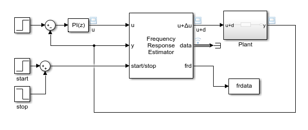
Offline — The block collects experiment data only and does not compute the estimated frequency response. You can get the experiment data at the data port (see that port description for more information). You can then perform the frequency-response estimation offline. For instance, you can use the data in MATLAB to compute the estimated frequency response with the
frestimatecommand. For more information, see Collect Frequency Response Experiment Data for Offline Estimation.
Programmatic Use
Block Parameter:
EstimationMode |
| Type: character vector, string |
Values:
'Online' | 'Offline'
|
Default:
'Online' |
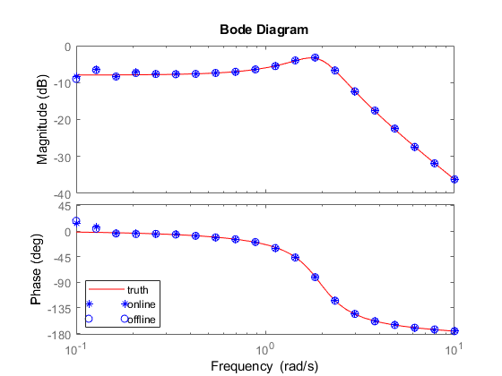
Select to generate a Bode plot showing the estimated frequency response. The plot updates periodically during the estimation experiment. If you have an LTI model representing the expected plant response or other relevant baseline, include it on the plot for reference using the Baseline plant model parameter.
Tips
To speed up trimming or linearization of a model containing a Frequency Response Estimator block, clear this parameter.
Programmatic Use
Block Parameter:
UseBodePlot |
| Type: character vector, string |
Values:
'off' | 'on'
|
Default:
'off' |
Specify the baseline model to plot with the estimated frequency response. Use an LTI
model such as a tf, ss, or
frd model.
Example: tf(10,[1 10 1000])
Dependencies
To enable this parameter, select Display Bode plot.
Programmatic Use
Block Parameter:
BaselinePlant |
| Type: LTI model |
Default:
'[]' |
During the frequency response estimation experiment, the block updates the Bode plot with the estimated frequency responses as often as you specify with this parameter. Increase the value if refreshing the Bode plot takes too much time.
For PRBS mode, the estimation happens at the end of the experiment, therefore, the bode plot is only updated once.
Dependencies
To enable this parameter, select Display Bode plot.
Programmatic Use
Block Parameter:
PlotRefreshFactor |
| Type: integer |
Default:
'100' |
More About
The block supplies the perturbation Δu for the duration of the experiment (while the start/stop signal is positive). The block determines how long to wait for system transients to die away and how many cycles to use for estimation as shown in the following illustration.
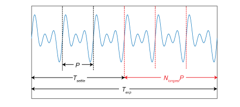
Texp is the experiment duration that you specify with your configuration of the start/stop signal (See the start/stop port description on the block reference page for more information). For the estimation computation, the block uses only the data collected in a window of NlongestP. Here, P is the period of the slowest frequency in the frequency vector ω, and Nlongest is the value of the Number of periods of the lowest frequency used for estimation block parameter. Any cycles before this window are discarded. Thus, the settling time Tsettle = Texp – NlongestP. If you know that your system settles quickly, you can shorten Texp without changing Nlongest to effectively shorten Tsettle. If your system is noisy, you can increase Nlongest to get more averaging in the data-collection window. Either way, always choose Texp long enough for sufficient settling and sufficient data-collection. The recommended Texp = 2NlongestP.
Algorithms
When Experiment mode is Sinestream, the block uses a correlation analysis method. In this method, the measured plant output y(t) is mixed with a sine signal and a cosine signal at the test frequency ω. The resulting signal is then integrated and averaged for a time T = N(2π/ω), where N is the integer value of the Number of estimation periods parameter. These operations are shown in the following diagram.

As the averaging time T increases, the contribution of components in y(t) at frequencies other than ω go to zero. R(T) and I(T) become constant and can be used to calculate the frequency response of the plant at ω. For further details, see [1].
References
[1] Wellstead, P. E. Technical Report 10: Frequency Response Analysis. Farnborough, Hampshire, UK: Solartron Instruments, 1997.