Deploy Frequency Response Estimation Algorithm for Real-Time Use
You can use the online frequency-response estimation algorithm in a standalone application for real-time estimation of a physical plant. To do so, you must deploy the Frequency Response Estimator block into your own system by creating a Simulink® model for deployment. You can configure this model with the experiment parameters. Or, you can configure it to supply such parameters externally from elsewhere in your system. Once deployed to your own system, the estimator model injects signals into your plant and receives the plant response, without using Simulink to control the experiment. Deploying the estimation algorithm requires a code-generation product such as Simulink Coder™.
Workflow
In overview, the workflow for deploying the Frequency Response Estimator for real-time tuning is:
Create a Simulink model for deploying the block to your system.
Configure the start/stop signal that controls when the estimation experiment begins and ends.
Configure experiment parameters such as the frequencies at which you want to perform estimation.
Deploy the model to your system, and run the estimation experiment against your physical plant. When you end the experiment, you can examine the estimated frequency response.
In practice, for real-time estimation, you might want to specify some parameters at run time, such as the estimation frequencies or perturbation amplitudes. For information about specifying parameters in your deployed application, see Access Experiment Parameters After Deployment.
Step 1. Create Deployable Simulink Model with Frequency Response Estimator Block
Using a Frequency Response Estimator block for real-time estimation requires creating a Simulink model for deployment. In the most basic form, a model for deploying real-time estimation resembles the following illustration.

Here, the blocks connected to the inputs and outputs of the Frequency Response Estimator block represent hardware interfaces that read or write real-time data for your system. For example, the Read control signal block can be an interface for receiving serial data, a UDP Receive block for receiving UDP packets, or an interface for receiving other signals via wireless network. Similarly the blocks for writing data, such as Write plant input, can be interfaces for serial, UDP, or other interfaces for writing data to hardware.
The default ports of the Frequency Response Estimator block are:
u— Receives the control signal.y— Receives the plant output.start/stop— Receives the signal that begins and ends the estimation experiment.u + Δu— Outputs the signal to feed to the plant input. When the experiment is not running,u + Δuoutputs the control signal as received atu. When the experiment is running, the block adds the perturbationΔuto this signal.data— Outputs the simulation data collected during the estimation experiment. This data includes the perturbation applied to the plant input and the response received aty.frd— Outputs the estimated frequency responses.
For more details about all ports, see the Frequency Response Estimator block reference page.
In the illustrated configuration, the frequencies at which to perform estimation and the amplitudes of the perturbation to apply at each frequency are hard-wired into the block. If you want to set these values after deployment, set the block parameter Excitation Signal Source to External ports. Doing so adds the w and amp ports to the block, as shown in the following illustration.
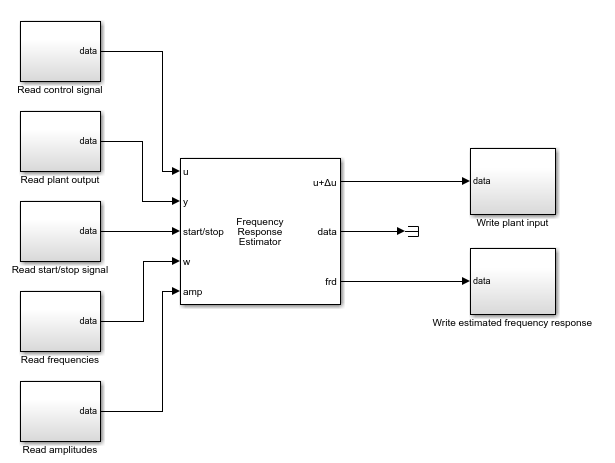
In this configuration, the deployed module can read frequencies and perturbation amplitudes for the estimation experiment at run time.
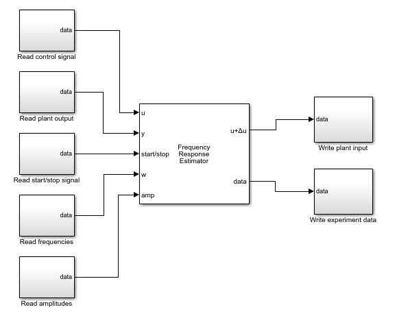
Store Data for Offline Estimation
The previously illustrated configurations discard the data output port,
which provides the input and response signals collected during the estimation
experiment. If you want to use this experiment data, you can store the output from
this port. For instance, to conserve resources in a deployed environment, you can
configure the block to collect the experiment data without performing the
estimation. You can then perform the estimation in MATLAB® using frestimate. A model configured
this way for deployment resembles the following illustration.
Step 2. Configure Start/Stop Signal
To start and stop the frequency response estimation experiment, use a signal at the start/stop port. When the experiment is not running, the block generates no perturbation signal. In this state, the block has no impact on plant behavior. The frequency-response estimation experiment begins and ends when the block receives a rising or falling signal at the start/stop port, respectively. You can configure any logic appropriate for your application to control the start and stop times of the experiment.
The block provides a recommended experiment length in the Experiment Length section of the block parameters. Typically, you configure the start/stop signal such that there is at least that much time between the rising and falling signals. In a deployed environment when you are setting estimation parameters at run time, you must be aware of how experiment parameters such as estimation frequencies affect the required experiment length. For more information about determining the appropriate length, see the Frequency Response Estimator block reference page.
Step 3. Set Experiment Parameters
The frequency-response estimation experiment injects signals at the frequencies you
specify with the Frequencies parameter (or at the w
port) of the Frequency Response Estimation block. Specify the perturbation
amplitudes using the Amplitudes parameter (or at the
amp port).
The block can apply the perturbation at each frequency as sequential sinusoidal (Sinestream), simultaneous sinusoidal (Superposition), or pseudorandom binary sequence (PRBS). To specify which mode to use, set the Experiment mode parameter.
Sinestream mode — Applies the perturbation one frequency at a time. Sinestream mode can be more accurate and can accommodate a wider range of frequencies than superposition mode.
Superposition — Applies the perturbation as a superposition signal containing all frequencies at once. The estimation experiment is generally faster in superposition mode.
PRBS — Applies the perturbation as a deterministic pseudorandom binary sequence that shifts between two values and has white-noise-like properties. PRBS signals reduce total estimation time compared to the other two modes, while producing comparable estimation results. PRBS signals are useful for estimating frequency responses for communications and power electronics systems.
You can also specify parameters that tell the block how long to let the system settle when the perturbation is applied, and how long to measure the response for the estimation. For further details about the two signal types and their relative advantages, see the Experiment mode parameter description on the Frequency Response Estimator block reference page.
Step 4. Run Experiment
After you deploy the estimation module to your system, use a rising
start/stop signal to begin the estimation experiment. The
deployed module injects the test signals into your physical plant in real time. After an
appropriate time, your falling start/stop signal ends the experiment.
(For more information about determining the appropriate length, see the Frequency Response
Estimator block reference page.)
When the experiment is complete, you can obtain the estimated frequency response at
the frd port.
If your deployed environment is short of resources for the online estimation computation, you can configure the block to collect experiment data only, and perform the estimation offline later. For an example, see Collect Frequency Response Experiment Data for Offline Estimation.
Access Experiment Parameters After Deployment
Some of the parameters that you set to configure the estimation experiment are tunable, such that you can access them in the generated code. Most parameters, however, are not tunable. For those parameters, you must configure them in the block before deployment, or use an external block port for the parameters for which one is available.
Tunable Parameters
The following parameters of the Frequency Response Estimator block are tunable after deployment. For more information about all these parameters, see the block reference pages.
| Parameter | Description |
|---|---|
| Number of estimation periods | Number of periods after settling to use for estimation (sinestream mode) |
| Number of settling periods | Number of periods to wait for settling of transients (sinestream mode) |
| Number of periods of the lowest frequency used for estimation | Duration of data-collection window (superposition mode) |
Non-Tunable Parameters
The remaining parameters of the Frequency Response Estimator are not tunable after deployment. For the Frequencies and Amplitudes parameters, you can enable external ports that allow you to supply experiment frequencies and perturbation amplitudes after deployment. To enable the w and amp block inputs, in the Excitation Signal Source parameter, select External ports.
Modify Experiment Sample Time After Deployment
The Sample time (Ts) parameter is not tunable. As a consequence, you cannot access it directly in generated code when you deploy the block. To change the controller sample time in the deployed block at run time:
Set Controller sample time (sec) to –1.
Put the block in a Triggered Subsystem.
Trigger the subsystem at the desired sample time.
If you use this approach, you must make sure at run time that your sample time is fast enough to keep your estimation frequencies below the Nyquist frequency.