Collect Frequency Response Experiment Data for Offline Estimation
This example shows how to use the Frequency Response Estimator block to perform a frequency response estimation experiment and store the data for later estimation offline. In practice, you can use this approach to perform the experiment in real time against a physical plant, when your deployed environment is short of resources for the online estimation computation. In this example, for illustration purposes, you perform the experiment on a plant modeled in Simulink®.
Model and Experiment Parameters
This example uses a model that already contains a Frequency Response Estimator block configured to collect experiment data for offline estimation.
Open the model.
mdl = "CollectFreqRespEstimDataEx.slx";
open_system(mdl)
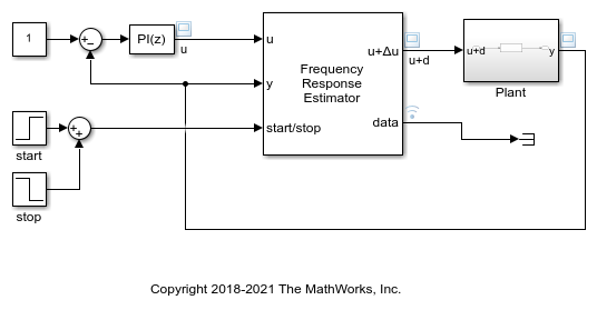
The model contains a plant in a closed-loop configuration with a PI controller. The Frequency Response Estimator block accepts the control signal as the input u. It feeds the control signal plus a perturbation into the plant input.
The Frequency Response Estimator block is configured to run the experiment in sinestream mode, with the same experiment parameters used in the example Online Frequency Response Estimation During Simulation. In this example, however, the Estimation Mode parameter is set to Offline. In this configuration, the block injects the specified perturbation signals and collects the response data, but does not perform the estimation. The block is configured to use a sinestream signal at the frequencies w = logspace(0,2,20).
Collect Experiment Data
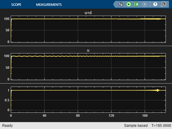
Simulate the model. The block performs the experiment and collects the response data. The scope shows the applied sinestream signal and the system response.
sim(mdl)
open_system('CollectFreqRespEstimDataEx/Scope1')
The model is configured to log the estimation data at the block output port data (see Save Signal Data Using Signal Logging for information about data logging). The data is stored in the MATLAB workspace as the Simulink.SimulationData.Dataset object logsout. Because data is the only logged port, you can access the logged data in the first entry in logsout. The Values field of that entry is a structure containing four fields.
logdata = logsout{1}.Values
logdata =

  struct with fields:

           Ready: [1×1 timeseries]
    Perturbation: [1×1 timeseries]
      PlantInput: [1×1 timeseries]
     PlantOutput: [1×1 timeseries]
            Info: [1×1 struct]
               u: [1×1 timeseries]
               y: [1×1 timeseries]
The Ready field is a timeseries containing a logical signal that indicates which time steps contain the data to used for the estimation. For a sinestream signal, this field indicates which perturbation periods for the estimation to discard (settling periods). Perturbation contains the sinestream perturbation applied to the plant. The PlantInput and PlantOutput timeseries contain the signals at the block inputs u and y, respectively.
Estimate Frequency Response
If you collect this data in a deployed environment with limited computational resources, you can use the data to perform frequency response estimation offline, using the frestimate command. Give frestimate the logdata structure and the same frequencies you used for the Frequencies parameter in the block. frestimate processes logdata to obtain a frequency response data (frd) model containing the estimated responses at those frequencies.
sys_estim = frestimate(logdata,w,'rad/s');
size(sys_estim)
FRD model with 1 outputs, 1 inputs, and 20 frequency points.
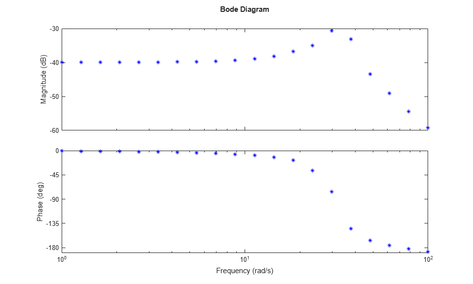
Examine the estimated frequency response.
figure
bode(sys_estim,'b*')