Online Estimation of Frequency Responses of a Nonlinear Plant
This example shows how to use the Frequency Response Estimator block to perform online estimation of the plant frequency responses. For a nonlinear plant, estimation at different nominal operating points produces different frequency responses.
Real Time Frequency Response Estimation
Frequency response describes the steady state response of a system to a sinusoidal input signal. If the system is linear  (
( ), the output signal is a sine wave of the same frequency with a different magnitude and a phase shift. A frequency response data (
frd) model that stores frequency response information at multiple frequencies is useful for tasks such as analyzing plant dynamics, validating linearization results, designing a control system, and estimating a parametric model.
There are different ways to obtain an frd model in the Simulink® environment. The most common approach is to linearize the Simulink model and calculate the frequency responses directly from the obtained state-space system. When the Simulink model cannot be linearized, you can use the frestimate command or use the Model Linearizer app to run simulation with some perturbation signals. Afterwards, the plant frequency responses are estimated offline based on the collected experiment data. This approach is called offline estimation.
This example shows an alternative online estimation approach using the Frequency Response Estimator block is to conduct an experiment and estimate the frequency response during simulation. Although this example uses a plant modeled in Simulink, if you do not have a plant model in Simulink, you can deploy the block on your target system and carry out frequency response estimation against a physical plant in real time. For more information, see Online Frequency Response Estimation Basics.
Nonlinear Plant Model
This example uses a stable nonlinear SISO plant. The plant has two states. Trim the model to find an initial steady-state operating point at which the plant output is zero.
plantMDL = 'scdfrePlant';
y0 = 0;
op = operspec(plantMDL);
op.Outputs.Known = true;
op.Outputs.y = y0;
options = findopOptions('DisplayReport','off');
[op_point, op_report] = findop(plantMDL,op,options);
x0 = [op_report.States(1).x;op_report.States(2).x];
y0 = op_report.Outputs.y;
u0 = op_report.Inputs.u;
A goal of this example is to obtain plant frequency responses from 0.1 rad/s to 10 rad/s at two other steady-state operating points, plant output = 0.5 and plant output = -0.5. To bring the plant to these operating points, design a discrete PID controller at the initial operating point. Use a controller sample time of 0.01 sec and an open-loop bandwidth is 20 rad/s.
Ts = 0.01;
G0 = c2d(linearize(plantMDL,op_point),Ts);
c = pidtune(G0,'pidf',20);
Online Estimation Using Sinestream Mode
The model scdfreSinestream includes the plant in a PID control loop using the controller c. It also contains the Frequency Response Estimator block in the control action + perturbation output configuration. In that configuration, you insert the block into the control loop between controller and plant.
mdlSS = 'scdfreSinestream';
open_system(mdlSS);
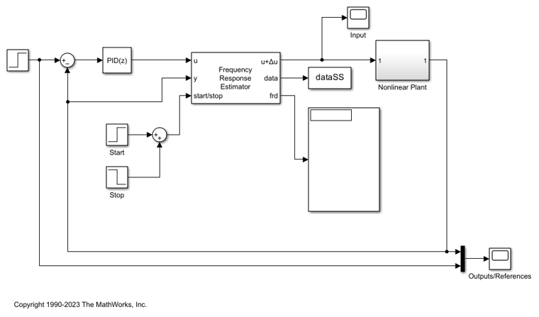
You can use the start/stop signal to start and stop an online estimation experiment. When the block is idle, the control signal passes through the block without any change.
During the experiment, when the Experiment Mode is Sinestream, the block injects sinusoidal signals into to the plant one frequency after another, from the lowest to the highest. Compared with the Superposition mode, the sinestream experiment is less intrusive and more accurate. However, it requires a much longer time to conduct the experiment.
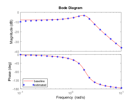
In this example, you can obtain an exact linearization of the model. Therefore, you can use it as the baseline in the block, letting you directly compare estimation result with this "truth" at run time. Find a steady-state operating point at which the plant output is 0.5, and linearize at this operating point to obtain G1.
op.Outputs.y = 0.5;
op_point = findop(plantMDL,op,options);
G1 = c2d(linearize(plantMDL,op_point),Ts);
Configure the block to use the model G1 as the baseline for the Bode plot.
set_param([mdlSS,'/Frequency Response Estimator'], 'BaselinePlant', 'G1');
The experiment starts at 10 sec after PID controller moves the plant to the new operating point (y = 0.5). After the experiment starts, the PID controller tries to reject the injected sine waves, which are effectively load disturbance. Thus the controller ensures that the plant does not move too far away from the nominal operating point during the experiment, and reduces the impact of plant nonlinearity on the estimation result. Simulate the model and observe on the Bode plot how the estimated response evolves during the experiment. The estimation result matches the baseline very well.
sim(mdlSS);
figSS = gcf;
hold on;

Online Estimation Using Superposition Mode
Open another model, scdfreSuperposition. In this model, the Frequency Response Estimator block is configured for perturbation only output. In this configuration, you can position to block outside of the control loop. When the block is idle, the perturbation signal entering the Sum block is 0, so the loop is unaffected.
mdlSP = 'scdfreSuperposition';
open_system(mdlSP);

This model has the same plant and controller. However, the Frequency Response Estimator block in this model is configured to use the Superposition experiment mode. In this mode, all the sine waves are added together and injected to the plant at the same time. Compared with the sinestream experiment, the superposition experiment is must faster (especially when you are targeting low frequencies).
Find a steady-state operating point with plant output of -0.5. Linearize the plant to find a baseline response at this operating point, G2.
op.Outputs.y = -0.5;
op_point = findop(plantMDL,op,options);
G2 = c2d(linearize(plantMDL,op_point),Ts);
Configure the block to use the model G2 as the baseline for the Bode plot.
set_param([mdlSP,'/Frequency Response Estimator'], 'BaselinePlant', 'G2');
The experiment starts at 10 sec after the PID controller moves the plant to the new operating point (y = -0.5). Note that the recommended experiment length is 377 seconds, much shorter than 1738 seconds used in the sinestream experiment. Simulate the model and again observe the progress of the estimation on the Bode plot.
sim(mdlSP);
figSP = gcf;
hold on;
Online Estimation Using PRBS Mode
Open another model, scdfrePRBS. In this model, the Frequency Response Estimator block is configured for perturbation only output. In this configuration, you can position to block outside of the control loop. When the block is idle, the perturbation signal entering the Sum block is 0, so the loop is unaffected.
mdlPRBS = 'scdfrePRBS';
open_system(mdlPRBS);
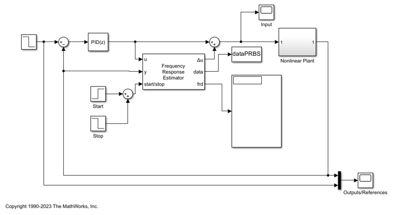
This model has the same plant and controller. However, the Frequency Response Estimator block in this model is configured to use the PRBS experiment mode. In this mode, a pseudorandom binary sequence is injected into the plant model. Compared with the sinestream and superposition experiments, the PRBS experiment is much faster even with much higher resolution in frequency domain.
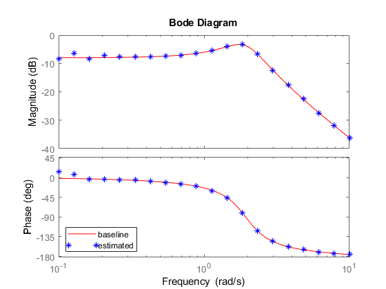
Find a steady-state operating point with plant output of -0.5. Linearize the plant to find a baseline response at this operating point, G3.
op.Outputs.y = -0.5;
op_point = findop(plantMDL,op,options);
G3 = c2d(linearize(plantMDL,op_point),Ts);
Configure the block to use the model G3 as the baseline for the Bode plot.
set_param([mdlPRBS,'/Frequency Response Estimator'], 'BaselinePlant', 'G3');
The experiment starts at 10 sec after the PID controller moves the plant to the new operating point (y = -0.5). Note that the recommended experiment length is 163.82 seconds, much shorter than 377 seconds used in the superposition experiment. Simulate the model and again observe the progress of the estimation on the Bode plot.
sim(mdlPRBS);
figPRBS = gcf;
hold on;
Offline Estimation Using Logged Experiment Data
Frequency Response Estimator block has a data outport that allows you to log the experiment data from simulation or in real-time. You can process that data set offline with the frestimate command to generate an frd object.
w = logspace(-1,1,20);
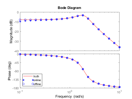
Compare online and offline estimation results from the sinestream experiment.
G1frd = frestimate(dataSS,w,'rad/s');
figure(figSS);
bodeplot(gca,G1frd,w,'o');
legend('truth','online','offline')

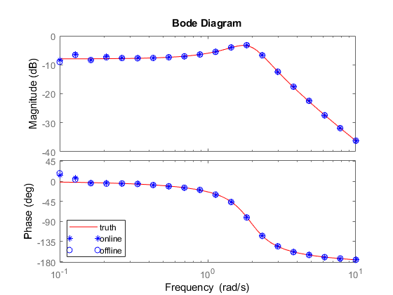
Compare online and offline estimation results from the superposition experiment.
G2frd = frestimate(dataSP,w,'rad/s');
figure(figSP);
bodeplot(gca,G2frd,w,'o');
legend('truth','online','offline')
Compare online and offline estimation results from the PRBS experiment.
G3frd = frestimate(dataPRBS,w,'rad/s');
figure(figPRBS);
bodeplot(gca,G3frd,w,'o');
legend('truth','online','offline')
For more information about using experiment data for offline estimation, see Collect Frequency Response Experiment Data for Offline Estimation.