FIR Filter Design

This example shows how to use windowing, least squares, or the Parks-McClellan algorithm to design lowpass, highpass, multiband, or arbitrary-response filters, differentiators, or Hilbert transformers.

FIR vs. IIR Filters

Digital filters with finite-duration impulse response (all-zero, or FIR filters) have both advantages and disadvantages compared to infinite-duration impulse response (IIR) filters. FIR filters have the following primary advantages:

• They can have exactly linear phase.

• They are always stable.

• The design methods are generally linear.

• They can be realized efficiently in hardware.

• The filter startup transients have finite duration.

The primary disadvantage of FIR filters is that they often require a much higher filter order than IIR filters to achieve a given level of performance. Correspondingly, the delay of these filters is often much greater than for an equal performance IIR filter.

FIR Filter Summary

The following table summarizes the various filter design methods using Signal Processing Toolbox™ and lists the functions available to implement these methods.

Filter Design Method	Description	Filter Functions
Windowing	Apply window to truncated inverse Fourier transform of specified "brick wall" filter	fir1, fir2, kaiserord
Multiband with Transition Bands	Equiripple or least squares approach over sub-bands of the frequency range	firls, firpm, firpmord
Constrained Least Squares	Minimize squared integral error over entire frequency range subject to maximum error constraints	fircls, fircls1
Arbitrary Response	Arbitrary responses, including nonlinear phase and complex filters	cfirpm
Raised Cosine	Lowpass response with smooth, sinusoidal transition	rcosdesign

You can also design digital filters with digitalFilter objects. See designfilt for or more information.

For a GUI-based workflow, use the Filter Designer app or the Design Filter live task to design filters.

Linear Phase Filters

Except for cfirpm, all of the FIR filter design functions design linear phase filters only. The filter coefficients, or “taps,” of such filters obey either an even or odd symmetry relation. Depending on this symmetry, and on whether the order n of the filter is even or odd, a linear phase filter (stored in length $\mathit{n}+1$vector b) has certain inherent restrictions on its frequency response.

Linear Phase Filter Type	Filter Order	Symmetry of Coefficients $$\left(\mathit{k}=1,...,\mathit{n}+1\right)$$	Response $\mathit{H}\left(\mathit{f}\right)$, $\mathit{f}=0$	Response $\mathit{H}\left(\mathit{f}\right)$, $\mathit{f}=1$ (Nyquist)
Type I	Even	Even: $\mathit{b}\left(\mathit{k}\right)=\mathit{b}\left(\mathit{n}+2-\mathit{k}\right)$	No restriction	No restriction
Type II	Odd	Even: $\mathit{b}\left(\mathit{k}\right)=\mathit{b}\left(\mathit{n}+2-\mathit{k}\right)$	No restriction	$$\mathit{H}\left(1\right)=0$$
Type III	Even	Odd: $\mathit{b}\left(\mathit{k}\right)=-\mathit{b}\left(\mathit{n}+2-\mathit{k}\right)$	$$\mathit{H}\left(0\right)=0$$	$$\mathit{H}\left(1\right)=0$$
Type IV	Odd	Odd: $\mathit{b}\left(\mathit{k}\right)=-\mathit{b}\left(\mathit{n}+2-\mathit{k}\right)$	$\mathit{H}\left(0\right)=0$	No restriction

The phase delay and group delay of linear phase FIR filters are equal and constant over the frequency band. For an order n linear phase FIR filter, the group delay is $\mathit{n}/2$, and the filtered signal is simply delayed by $\mathit{n}/2$ time steps (and the magnitude of its Fourier transform is scaled by the filter's magnitude response). This property preserves the wave shape of signals in the passband; that is, there is no phase distortion.

The functions fir1, fir2, firls, firpm, fircls, and fircls1 all design type I and II linear phase FIR filters by default. rcosdesign designs only type I filters. Both firls and firpm design type III and IV linear phase FIR filters given a "hilbert" or "differentiator" flag. cfirpm can design any type of linear phase filter, and nonlinear phase filters as well.

Because the frequency response of a type II filter is zero at the Nyquist frequency (“high” frequency), fir1 does not design type II highpass and bandstop filters. For odd-valued n in these cases, fir1 adds 1 to the order and returns a type I filter.

Windowing Method

Consider the ideal, or “brick wall,” digital lowpass filter with a cutoff frequency of ${\omega }_0$ rad/sample. This filter has magnitude 1 at all frequencies with magnitude less than ${\omega }_0$, and magnitude 0 at frequencies with magnitude between ${\omega }_0$ and $\pi$. Its impulse response sequence $\mathit{h}\left(\mathit{n}\right)$ is

$$\mathit{h}\left(\mathit{n}\right)=\frac{1}{2\pi }{\int }_{-\pi }^{\pi }\mathit{H}\left(\omega \right){\mathit{e}}^{\mathit{j}\omega \mathit{n}}\mathit{d}\omega =\frac{1}{2\pi }{\int }_{-{\omega }_0}^{{\omega }_0}{\mathit{e}}^{\mathit{j}\omega \mathit{n}}\mathit{d}\omega =\frac{\sin \left({\omega }_0\mathit{n}\right)}{\pi \mathit{n}}$$

This filter is not implementable since its impulse response is infinite and noncausal. To create a finite-duration impulse response, truncate it by applying a window. By retaining the central section of impulse response in this truncation, you obtain a linear phase FIR filter. For example, a length 51 filter with a lowpass cutoff frequency ${\omega }_0$ of 0.4 π rad/sample is

b = 0.4*sinc(0.4*(-25:25));

The window applied here is a simple rectangular window. By Parseval’s theorem, this is the length 51 filter that best approximates the ideal lowpass filter, in the integrated least squares sense. Display the filter frequency response. Note that the y-axis shown in the below is in magnitude squared.

filterAnalyzer(b,MagnitudeMode="squared")

Ringing and ripples occur in the response, especially near the band edge. This “Gibbs effect” does not vanish as the filter length increases, but a nonrectangular window reduces its magnitude. Multiplication by a window in the time domain causes a convolution or smoothing in the frequency domain. Apply a length 51 Hamming window to the filter and display the result. Note that the $\mathit{y}$-axis shown in the figure is in magnitude squared.

bw = b.*hamming(51)';
filterAnalyzer(bw,MagnitudeMode="squared")

Using a Hamming window greatly reduces the ringing. This improvement is at the expense of transition width (the windowed version takes longer to ramp from passband to stopband) and optimality (the windowed version does not minimize the integrated squared error).

Standard Band FIR Filter Design: fir1

The fir1 function uses a least-squares approximation to compute filter coefficients and then smooths the impulse response with a window. For an overview of windows and their properties, see Windows. fir1 resembles the IIR filter design functions in that it is formulated to design filters in standard band configurations: lowpass, bandpass, highpass, and bandstop.

Create a row vector containing the coefficients of a 50th order Hamming-windowed lowpass filter.

n = 50;
Wn = 0.4;
bF1 = fir1(n,Wn);

This is a lowpass, linear phase FIR filter with cutoff frequency Wn. Wn is a number between 0 and 1, where 1 corresponds to the Nyquist frequency, half the sampling frequency. (Unlike other methods, here Wn corresponds to the 6 dB point.) For a highpass filter, simply append "high" to the function's parameter list. For a bandpass or bandstop filter, specify Wn as a two-element vector containing the passband edge frequencies. Append "stop" for the bandstop configuration.

bF1w = fir1(n,Wn,window) uses the window specified in column vector window for the design. The vector window must be n+1 elements long. If you do not specify a window, fir1 applies a Hamming window.

Kaiser Window Order Estimation

The kaiserord function estimates the filter order, cutoff frequency, and Kaiser window beta parameter needed to meet a given set of specifications. Given a vector of frequency band edges and a corresponding vector of magnitudes, as well as maximum allowable ripple, kaiserord returns appropriate input parameters for the fir1 function.

Multiband FIR Filter Design: fir2

The fir2 function also designs windowed FIR filters, but with an arbitrarily shaped piecewise linear frequency response. This is in contrast to fir1, which only designs filters in standard lowpass, highpass, bandpass, and bandstop configurations.

Generate a row vector b containing the n+1 coefficients of the order n FIR filter whose frequency-magnitude characteristics match those given by vectors f and m.

n = 50;
f = [0 .4 .5 1];
m = [1  1  0 0];
bF2 = fir2(n,f,m);
filterAnalyzer(bF2,MagnitudeMode="squared")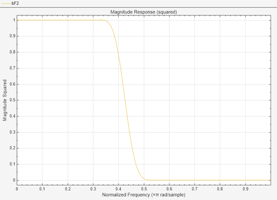

f is a vector of frequency points ranging from 0 to 1, where 1 represents the Nyquist frequency. m is a vector containing the specified magnitude response at the points specified in f. (The IIR counterpart of this function is yulewalk, which also designs filters based on arbitrary piecewise linear magnitude responses. See IIR Filter Design for details.)

Multiband FIR Filter Design with Transition Bands

The firls and firpm functions provide a more general means of specifying the ideal specified filter than the fir1 and fir2 functions. These functions design Hilbert transformers, differentiators, and other filters with odd symmetric coefficients (type III and type IV linear phase). They also let you include transition or “don't care” regions in which the error is not minimized, and perform band dependent weighting of the minimization.

The firls function is an extension of the fir1 and fir2 functions in that it minimizes the integral of the square of the error between the specified frequency response and the actual frequency response.

The firpm function implements the Parks-McClellan algorithm, which uses the Remez exchange algorithm and Chebyshev approximation theory to design filters with optimal fits between the specified and actual frequency responses. The filters are optimal in the sense that they minimize the maximum error between the specified frequency response and the actual frequency response; they are sometimes called minimax filters. Filters designed in this way exhibit an equiripple behavior in their frequency response, and hence are also known as equiripple filters. The Parks-McClellan FIR filter design algorithm is perhaps the most popular and widely used FIR filter design methodology.

The syntax for firls and firpm is the same; the only difference is their minimization schemes. The next example shows how filters designed with firls and firpm reflect these different schemes.

Basic Configurations

The default mode of operation of firls and firpm is to design type I or type II linear phase filters, depending on whether the order you want is even or odd, respectively. A lowpass example with approximate amplitude 1 from 0 to 0.4 Hz, and approximate amplitude 0 from 0.5 to 1.0 Hz is

n0 = 20;               % Filter order
f0 = [0 0.4 0.5 1];    % Frequency band edges
A0 = [1  1  0 0];      % Amplitudes
bPM0 = firpm(n,f0,A0);

From 0.4 to 0.5 Hz, firpm performs no error minimization; this is a transition band or “don't care” region. A transition band minimizes the error more in the bands that you do care about, at the expense of a slower transition rate. In this way, these types of filters have an inherent trade-off similar to FIR design by windowing.

To compare least squares to equiripple filter design, use firls to create a similar filter. Type

bLS0 = firls(n0,f0,A0);

and compare their frequency responses using Filter Analyzer. Note that the y-axis shown in the figure below is in magnitude squared. You can set this automatically by using the name-value argument MagnitudeMode, or manually by clicking on the Analysis Options button in the Analyzer section and selecting Squared from the Magnitude Options menu in the Filter Analyzer app.

filterAnalyzer(bPM0,1,bLS0,1, ...
    FilterNames=["bPM0" "bLS0"],MagnitudeMode="squared")

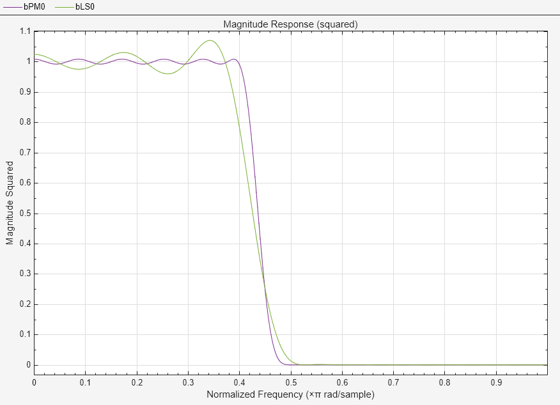
The filter designed with firpm exhibits equiripple behavior. Also note that the firls filter has a better response over most of the passband and stopband, but at the band edges (f = 0.4 and f = 0.5), the response is further away from the ideal than the firpm filter. This shows that the firpm filter's maximum error over the passband and stopband is smaller and, in fact, it is the smallest possible for this band edge configuration and filter length.

Think of frequency bands as lines over short frequency intervals. firpm and firls use this scheme to represent any piecewise linear frequency-response function with any transition bands. firls and firpm design lowpass, highpass, bandpass, and bandstop filters; a bandpass example is

fMB0 = [0 0.3  0.4  0.7  0.8  1]; % Band edges in pairs
aMB0 = [0  0    1    1    0   0]; % Bandpass filter amplitude

Technically, these f and a vectors define five bands:

• Two stopbands, from 0.0 to 0.3 and from 0.8 to 1.0

• A passband from 0.4 to 0.7

• Two transition bands, from 0.3 to 0.4 and from 0.7 to 0.8

Example highpass and bandstop filters are

fHP = [0 0.7  0.8  1];           % Band edges in pairs
aHP = [0  0    1   1];           % Highpass filter amplitude
fBS = [0 0.3  0.4  0.5  0.8  1]; % Band edges in pairs
aBS = [1  1    0    0    1   1]; % Bandstop filter amplitude

An example multiband bandpass filter is

fMB = [0 0.1 0.15 0.25 0.3 0.4 0.45 0.55 0.6 0.7 0.75 0.85 0.9 1];
aMB = [1  1   0    0    1   1   0    0    1   1   0    0    1  1];

Another possibility is a filter that has as a transition region the line connecting the passband with the stopband; this can help control “runaway” magnitude response in wide transition regions:

fTB = [0 0.4 0.42 0.48 0.5  1];
aTB = [1 1 0.8 0.2 0 0];   % Passband, linear transition, 
                         %  stopband

The Weight Vector

Both firls and firpm allow you to place more or less emphasis on minimizing the error in certain frequency bands relative to others. To do this, specify a weight vector following the frequency and amplitude vectors. An example lowpass equiripple filter with 10 times less ripple in the stopband than the passband is

nWV = 20;              % Filter order
fWV = [0 0.4 0.5 1];   % Frequency band edges
aWV = [1  1   0  0];   % Amplitudes
wv = [1 10];          % Weight vector
bWV = firpm(nWV,fWV,aWV,wv);

Anti-Symmetric Filters and Hilbert Transformers

When called with a trailing "h" or "hilbert" option, firpm and firls design FIR filters with odd symmetry, that is, type III (for even order) or type IV (for odd order) linear phase filters. An ideal Hilbert transformer has this anti-symmetry property and an amplitude of 1 across the entire frequency range. Try the following approximate Hilbert transformers and plot them.

bHHP = firpm(21,[0.05 1],[1 1],"hilbert");    % Highpass
bHBP = firpm(20,[0.05 0.95],[1 1],"hilbert"); % Bandpass
filterAnalyzer(bHHP,1,bHBP,1,FilterNames=["bHHP" "bHBP"])

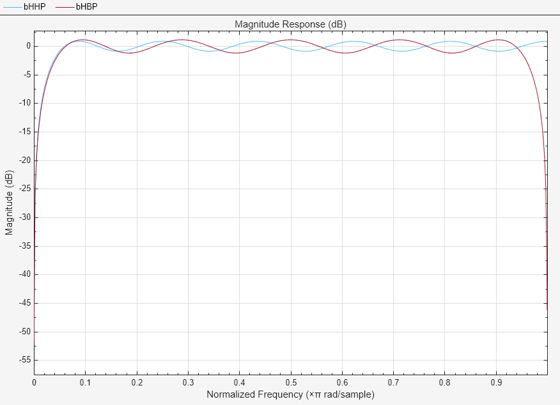
You can find the delayed Hilbert transform of a signal x by passing it through these filters.

fs = 1000;            % Sampling frequency
t = (0:1/fs:2)';      % Two second time vector
x = sin(2*pi*300*t);  % 300 Hz sine wave example signal
xh = filter(bHBP,1,x);  % Hilbert transform of x

The analytic signal corresponding to x is the complex signal that has x as its real part and the Hilbert transform of x as its imaginary part. For this FIR method (an alternative to the hilbert function), you must delay x by half the filter order to create the analytic signal:

xd = [zeros(10,1); x(1:length(x)-10)];	    % Delay 10 samples
xa = xd + 1i*xh;                            % Analytic signal

This method does not work directly for filters of odd order, which require a noninteger delay. In this case, the hilbert function, described in Hilbert Transform, estimates the analytic signal. Alternatively, use the resample function to delay the signal by a noninteger number of samples.

Differentiators

Differentiation of a signal in the time domain is equivalent to multiplication of the signal's Fourier transform by an imaginary ramp function. That is, to differentiate a signal, pass it through a filter that has a response $\mathit{H}\left(\omega \right)=\mathit{j}\omega$. Approximate the ideal differentiator (with a delay) using firpm or firls with a "d" or "differentiator" option:

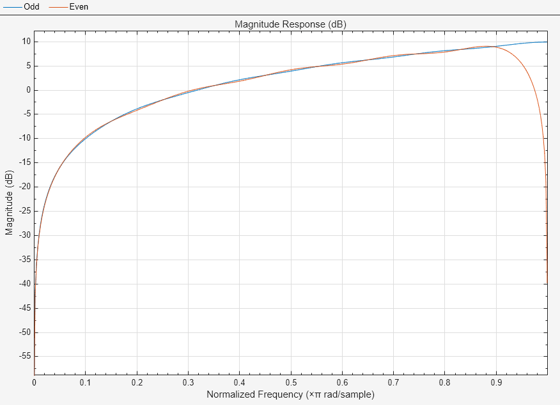
bDiff10 = firpm(21,[0 1],[0 pi],"differentiator");

For a type III filter, the differentiation band should stop short of the Nyquist frequency, and the amplitude vector must reflect that change to ensure the correct slope:

bDiff09 = firpm(20,[0 0.9],[0 0.9*pi],"differentiator");

In the "d" mode, firpm weights the error by $1/\omega$ in nonzero amplitude bands to minimize the maximum relative error. firls weights the error by ${\left(1/\omega \right)}^2$ in nonzero amplitude bands in the "d" mode.

The plot shows the magnitude responses for the differentiators.

filterAnalyzer(bDiff10,1,bDiff09,1,FilterNames=["Odd" "Even"])

Constrained Least Squares FIR Filter Design

The Constrained Least Squares (CLS) FIR filter design functions implement a technique that enables you to design FIR filters without explicitly defining the transition bands for the magnitude response. The ability to omit the specification of transition bands is useful in several situations. For example, it may not be clear where a rigidly defined transition band should appear if noise and signal information appear together in the same frequency band. Similarly, it may make sense to omit the specification of transition bands if they appear only to control the results of Gibbs phenomena that appear in the filter's response. See Selesnick, Lang, and Burrus [3] for discussion of this method.

Instead of defining passbands, stopbands, and transition regions, the CLS method accepts a cutoff frequency (for the highpass, lowpass, bandpass, or bandstop cases), or passband and stopband edges (for multiband cases), for the response you specify. In this way, the CLS method defines transition regions implicitly, rather than explicitly.

The key feature of the CLS method is that it enables you to define upper and lower thresholds that contain the maximum allowable ripple in the magnitude response. Given this constraint, the technique applies the least square error minimization technique over the frequency range of the filter's response, instead of over specific bands. The error minimization includes any areas of discontinuity in the ideal, "brick wall" response. An additional benefit is that the technique enables you to specify arbitrarily small peaks resulting from the Gibbs phenomenon.

There are two functions that implement this design technique.

Description	Function
Constrained least square multiband FIR filter design	fircls
Constrained least square filter design for lowpass and highpass linear phase filters	fircls1

For details on the calling syntax for these functions, see their reference descriptions in the Function Reference.

Basic Lowpass and Highpass CLS Filter Design

The most basic of the CLS design functions, fircls1, uses this technique to design lowpass and highpass FIR filters. As an example, consider designing a filter with order 61 impulse response and cutoff frequency of 0.3 (normalized). Further, define the upper and lower bounds that constrain the design process as:

• Maximum passband deviation from 1 (passband ripple) of 0.02.

• Maximum stopband deviation from 0 (stopband ripple) of 0.008.

To approach this design problem using fircls1, use the following commands:

n = 61;
wo = 0.3;
dp = 0.02;	
ds = 0.008;
bCLS = fircls1(n,wo,dp,ds);

Display the magnitude response. Note that the y-axis shown is in Magnitude Squared.

filterAnalyzer(bCLS,MagnitudeMode="squared")

Multiband CLS Filter Design

The fircls function uses the same technique to design FIR filters with a specified piecewise constant magnitude response. In this case, you can specify a vector of band edges and a corresponding vector of band amplitudes. In addition, you can specify the maximum amount of ripple for each band.

For example, assume the specifications for a filter call for:

• From 0 to 0.3 (normalized): amplitude 0, upper bound 0.005, lower bound –0.005

• From 0.3 to 0.5: amplitude 0.5, upper bound 0.51, lower bound 0.49

• From 0.5 to 0.7: amplitude 0, upper bound 0.03, lower bound –0.03

• From 0.7 to 0.9: amplitude 1, upper bound 1.02, lower bound 0.98

• From 0.9 to 1: amplitude 0, upper bound 0.05, lower bound –0.05

Design a CLS filter with impulse response order 129 that meets the specifications. Display the magnitude response. Note that the y-axis shown is in Magnitude Squared.

n = 129;
f = [0 0.3 0.5 0.7 0.9 1];
a = [0 0.5 0 1 0];
up = [0.005 0.51 0.03 1.02 0.05];
lo = [-0.005 0.49 -0.03 0.98 -0.05];
bCLSmb = fircls(n,f,a,up,lo);
filterAnalyzer(bCLSmb,MagnitudeMode="squared")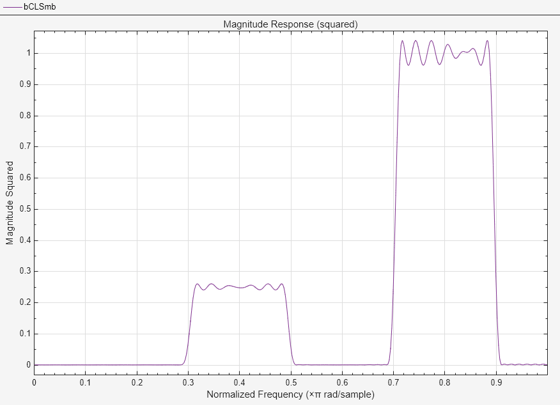

Weighted CLS Filter Design

Weighted CLS filter design lets you design lowpass or highpass FIR filters with relative weighting of the error minimization in each band. The fircls1 function enables you to specify the passband and stopband edges for the least squares weighting function, as well as a constant k that specifies the ratio of the stopband to passband weighting.

For example, consider specifications that call for an FIR filter with impulse response order of 55 and cutoff frequency of 0.3 (normalized). Also assume maximum allowable passband ripple of 0.02 and maximum allowable stopband ripple of 0.004. In addition, add weighting requirements:

• Passband edge for the weight function of 0.28 (normalized)

• Stopband edge for the weight function of 0.32

• Weight error minimization 10 times as much in the stopband as in the passband

To approach this using fircls1, type the following commands:. Note that the y-axis shown is in Magnitude Squared.

n = 55;
wo = 0.3;
dp = 0.02;
ds = 0.004;
wp = 0.28;
ws = 0.32;
k = 10;
bCLSw = fircls1(n,wo,dp,ds,wp,ws,k);
filterAnalyzer(bCLSw,MagnitudeMode="squared")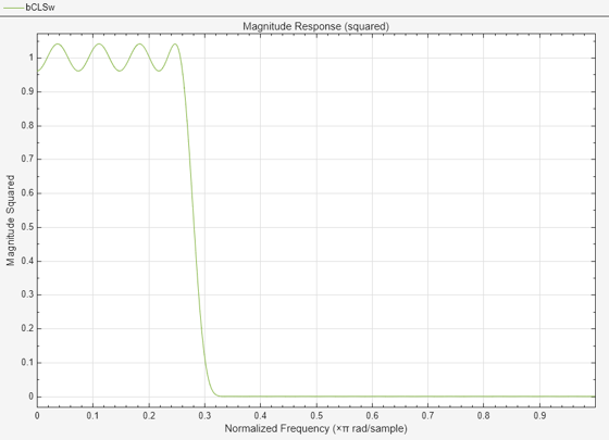

Arbitrary-Response Filter Design

The cfirpm filter design function provides a tool for designing FIR filters with arbitrary complex responses. It differs from the other filter design functions in how the frequency response of the filter is specified: it accepts the name of a function which returns the filter response calculated over a grid of frequencies. This capability makes cfirpm a highly versatile and powerful technique for filter design.

This design technique may be used to produce nonlinear-phase FIR filters, asymmetric frequency-response filters (with complex coefficients), or more symmetric filters with custom frequency responses.

The design algorithm optimizes the Chebyshev (or minimax) error using an extended Remez-exchange algorithm for an initial estimate. If this exchange method fails to obtain the optimal filter, the algorithm switches to an ascent-descent algorithm that takes over to finish the convergence to the optimal solution.

Multiband Filter Design

Consider a multiband filter with the following special frequency-domain characteristics.

Band	Amplitude	Optimization Weighting
$$\left[-1-0.5\right]$$	$$\left[51\right]$$	$$1$$
$$\left[-0.40.3\right]$$	$$\left[22\right]$$	$$10$$
$$\left[0.40.8\right]$$	$$\left[21\right]$$	$$5$$

A linear-phase multiband filter may be designed using the predefined frequency-response function multiband, as follows:

bMBh = cfirpm(38, [-1 -0.5 -0.4 0.3 0.4 0.8], ...
               {@multiband, [5 1 2 2 2 1]}, [1 10 5]);

For the specific case of a multiband filter, we can use a shorthand filter design notation similar to the syntax for firpm:

bMBd = cfirpm(38,[-1 -0.5 -0.4 0.3 0.4 0.8], ...
              [5 1 2 2 2 1], [1 10 5]);

As with firpm, a vector of band edges is passed to cfirpm. This vector defines the frequency bands over which optimization is performed; note that there are two transition bands, from –0.5 to –0.4 and from 0.3 to 0.4.

In either case, obtain the frequency response and plot using linear scale. Note that the range of data is (-pi,pi).

filterAnalyzer(bMBd,FrequencyRange="centered")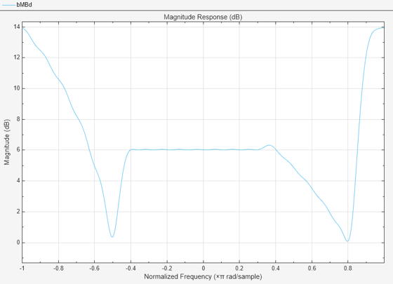

The filter response for this multiband filter is complex, which is expected because of the asymmetry in the frequency domain. The impulse response is shown below.

filterAnalyzer(bMBd,Analysis="impulse")

Filter Design with Reduced Delay

Consider the design of a 62-tap lowpass filter with a half-Nyquist cutoff. If we specify a negative offset value to the lowpass filter design function, the group delay offset for the design is significantly less than that obtained for a standard linear-phase design. This filter design may be computed as follows:

bRD = cfirpm(61,[0 0.5 0.55 1],{@lowpass,-16});

The resulting magnitude response is as follows. The y-axis is in Magnitude Squared, which you can set by right-clicking on the axis label and selecting Magnitude Squared from the menu.

filterAnalyzer(bRD,MagnitudeMode="squared")

The group delay of the filter reveals that the offset has been reduced from N/2 to N/2-16 (i.e., from 30.5 to 14.5). Now, however, the group delay is no longer flat in the passband region. To create this plot, click the Group Delay Response button on the toolbar.

filterAnalyzer(bRD,Analysis="groupdelay")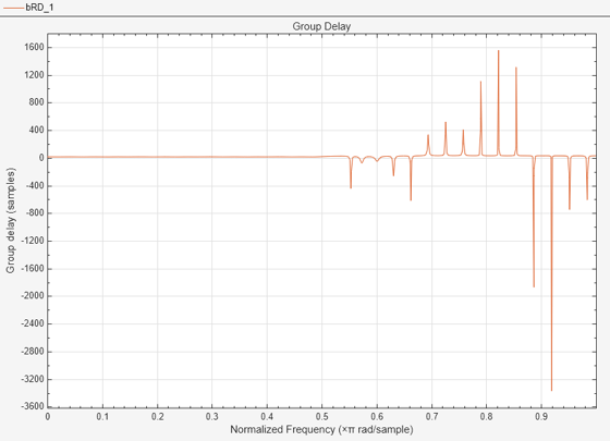

If we compare this nonlinear-phase filter to a linear-phase filter that has exactly 14.5 samples of group delay, the resulting filter is of order 2*14.5, or 29. Using bRD = cfirpm(29,[0 0.5 0.55 1],"lowpass"), the passband and stopband ripple is much greater for the order 29 filter. These comparisons can assist you in deciding which filter is more appropriate for a specific application.