fir2

Frequency sampling-based FIR filter design

Syntax

b = fir2(n,f,m)

b = fir2(n,f,m,npt,lap)

b = fir2(___,window)

Description

b = fir2(n,f,m) returns an nth-order FIR filter with frequency-magnitude characteristics specified in the vectors f and m. The function linearly interpolates the desired frequency response onto a dense grid and then uses the inverse Fourier transform and a Hamming window to obtain the filter coefficients.

b = fir2(n,f,m,npt,lap) specifies npt, the number of points in the interpolation grid, and lap, the length of the region that fir2 inserts around duplicate frequency points which specify steps in the frequency response.

b = fir2(___,window) specifies a window vector to use in the design in addition to any input arguments from previous syntaxes.

Note:   Use fir1 for window-based standard lowpass, bandpass, highpass, bandstop, and multiband configurations.

Examples

Attenuation of Low Frequencies

Load the MAT-file chirp. The file contains a signal, y, sampled at a frequency Fs = 8192 Hz. The signal has most of its power above Fs/4 = 2048 Hz, or half the Nyquist frequency. Add random noise to the signal.

load chirp
y = y + randn(size(y))/25;
t = (0:length(y)-1)/Fs;

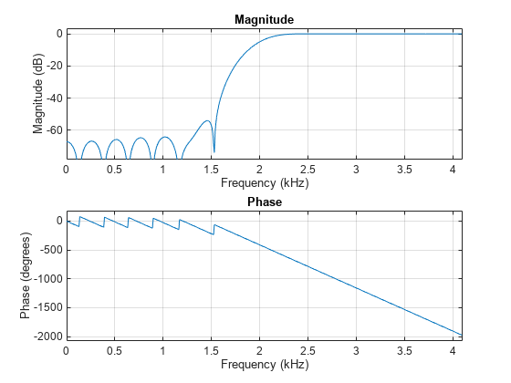
Design a 34th-order FIR highpass filter to attenuate the components of the signal below Fs/4. Specify a normalized cutoff frequency of 0.48, which corresponds to about 1966 Hz. Visualize the frequency response of the filter.

f = [0 0.48 0.48 1];
mhi = [0 0 1 1];
bhi = fir2(34,f,mhi);

freqz(bhi,1,[],Fs)

Filter the chirp signal. Plot the signal before and after filtering.

outhi = filter(bhi,1,y);

figure
subplot(2,1,1)
plot(t,y)
title('Original Signal')
ylim([-1.2 1.2])

subplot(2,1,2)
plot(t,outhi)
title('Highpass Filtered Signal')
xlabel('Time (s)')
ylim([-1.2 1.2])

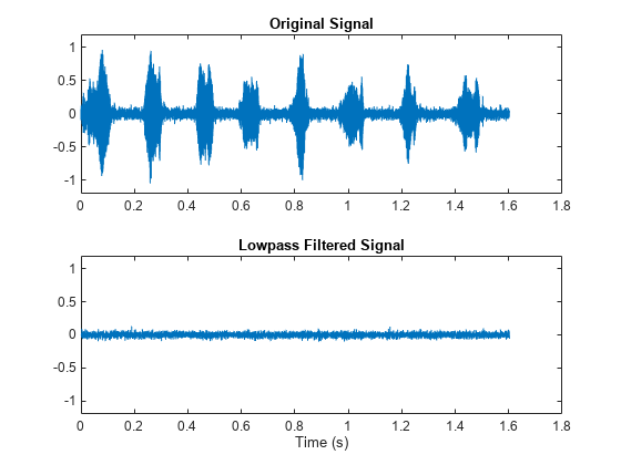
Change the filter from highpass to lowpass. Use the same order and cutoff. Filter the signal again. The result is mostly noise.

mlo = [1 1 0 0];
blo = fir2(34,f,mlo);
outlo = filter(blo,1,y);

subplot(2,1,1)
plot(t,y)
title('Original Signal')
ylim([-1.2 1.2])

subplot(2,1,2)
plot(t,outlo)
title('Lowpass Filtered Signal')
xlabel('Time (s)')
ylim([-1.2 1.2])

FIR Lowpass Filter

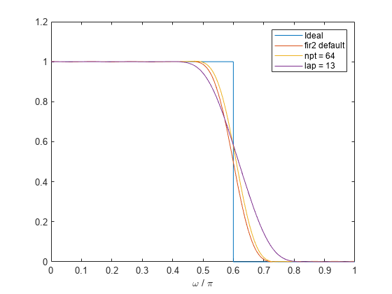
Design a 30th-order lowpass filter with a normalized cutoff frequency of $$0.6\pi$$ rad/sample. Plot the ideal frequency response overlaid with the actual frequency response.

f = [0 0.6 0.6 1];
m = [1 1 0 0];

b1 = fir2(30,f,m);
[h1,w] = freqz(b1,1);

plot(f,m,w/pi,abs(h1))
xlabel('\omega / \pi')
lgs = {'Ideal','fir2 default'};
legend(lgs)

Redesign the filter using a 64-point interpolation grid.

b2 = fir2(30,f,m,64);
h2 = freqz(b2,1);

hold on
plot(w/pi,abs(h2))
lgs{3} = 'npt = 64';
legend(lgs)

Redesign the filter using the 64-point interpolation grid and a 13-point interval around the cutoff frequency.

b3 = fir2(30,f,m,64,13);
h3 = freqz(b3,1);

plot(w/pi,abs(h3))
lgs{4} = 'lap = 13';
legend(lgs)

Arbitrary Magnitude Filter

Design an FIR filter with the following frequency response:

• A sinusoid between 0 and $$0.18\pi$$ rad/sample.

F1 = 0:0.01:0.18;
A1 = 0.5+sin(2*pi*7.5*F1)/4;

• A piecewise linear section between $$0.2\pi$$ rad/sample and $$0.78\pi$$ rad/sample.

F2 = [0.2 0.38 0.4 0.55 0.562 0.585 0.6 0.78];
A2 = [0.5 2.3 1 1 -0.2 -0.2 1 1];

• A quadratic section between $$0.79\pi$$ rad/sample and the Nyquist frequency.

F3 = 0.79:0.01:1;
A3 = 0.2+18*(1-F3).^2;

Design the filter using a Hamming window. Specify a filter order of 50.

N = 50;

FreqVect = [F1 F2 F3];
AmplVect = [A1 A2 A3];

ham = fir2(N,FreqVect,AmplVect);

Repeat the calculation using a Kaiser window that has a shape parameter of 3.

kai = fir2(N,FreqVect,AmplVect,kaiser(N+1,3));

Redesign the filter using the designfilt function. designfilt uses a rectangular window by default. Compute the zero-phase response of the filter over 1024 points.

d = designfilt('arbmagfir','FilterOrder',N, ...
    'Frequencies',FreqVect,'Amplitudes',AmplVect);

[zd,wd] = zerophase(d,1024);

Display the zero-phase responses of the three filters. Overlay the ideal response.

zerophase(ham,1)
hold on
zerophase(kai,1)
plot(wd/pi,zd)
plot(FreqVect,AmplVect,'k:')
legend('Hamming','Kaiser','designfilt','ideal')

Input Arguments

n — Filter order

integer scalar

Filter order, specified as an integer scalar.

For configurations with a passband at the Nyquist frequency, fir2 always uses an even order. If you specify an odd-valued n for one of those configurations, then fir2 increments n by 1.

Data Types: double

f,m — Frequency-magnitude characteristics

vectors

Frequency-magnitude characteristics, specified as vectors of the same length.

• f is a vector of frequency points in the range from 0 to 1, where 1 corresponds to the Nyquist frequency. The first point of f must be 0 and the last point must be 1. f must be sorted in increasing order. Duplicate frequency points are allowed and are treated as steps in the frequency response.

• m is a vector containing the desired magnitude response at each of the points specified in f.

Data Types: double

npt — Number of grid points

512 (default) | positive integer scalar

Number of grid points, specified as a positive integer scalar. npt must be larger than one-half the filter order: npt > n/2.

Data Types: double

lap — Length of region around duplicate frequency points

25 (default) | positive integer scalar

Length of region around duplicate frequency points, specified as a positive integer scalar.

Data Types: double

window — Window

column vector

Window, specified as a column vector. The window vector must have n + 1 elements. If you do not specify window, then fir2 uses a Hamming window. For a list of available windows, see Windows.

fir2 does not automatically increase the length of window if you attempt to design a filter of odd order with a passband at the Nyquist frequency.

Example: kaiser(n+1,0.5) specifies a Kaiser window with shape parameter 0.5 to use with a filter of order n.

Example: hamming(n+1) is equivalent to leaving the window unspecified.

Data Types: double

Output Arguments

b — Filter coefficients

row vector

Filter coefficients, returned as a row vector of length n + 1. The coefficients are sorted in descending powers of the Z-transform variable z:

B(z) = b(1) + b(2)z + … + b(n+1)z^–n.

Algorithms

fir2 uses frequency sampling to design filters. The function interpolates the desired frequency response linearly onto a dense, evenly spaced grid of length npt. fir2 also sets up regions of lap points around repeated values of f to provide steep but smooth transitions. To obtain the filter coefficients, the function applies an inverse fast Fourier transform to the grid and multiplies by window.

References

[1] Jackson, L. B. Digital Filters and Signal Processing. 3rd Ed. Boston: Kluwer Academic Publishers, 1996.

[2] Mitra, Sanjit K. Digital Signal Processing: A Computer Based Approach. New York: McGraw-Hill, 1998.

Extended Capabilities

C/C++ Code Generation

Generate C and C++ code using MATLAB® Coder™.

Usage notes and limitations:

All inputs must be constants. Expressions or variables are allowed if their values do not change.

Version History

Introduced before R2006a