Main Content

firls

Least-squares linear-phase FIR filter design

Description

b = firls(n,f,a) returns row vector b containing the n+1 coefficients of an order-n FIR filter. The frequency and amplitude characteristics of the resulting filter match those given by vectors f and a.

example

b = firls(n,f,a,w) uses w to weight the frequency bins.

example

b = firls(___,ftype) designs antisymmetric (odd) filters, where ftype specifies the filter as a differentiator or Hilbert transformer. You can use ftype with any of the previous input syntaxes.

example

Examples

collapse all

Design an FIR lowpass filter of order 255 with a transition region between 0.25π and 0.3π. Display the magnitude and phase responses of the filter.

b = firls(255,[0 0.25 0.3 1],[1 1 0 0]);
freqz(b,1)

Figure contains 2 axes objects. Axes object 1 with title Phase, xlabel Normalized Frequency (\times\pi rad/sample), ylabel Phase (degrees) contains an object of type line. Axes object 2 with title Magnitude, xlabel Normalized Frequency (\times\pi rad/sample), ylabel Magnitude (dB) contains an object of type line.

An ideal differentiator has a frequency response given by D(ω)=jω. Design a differentiator of order 30 that attenuates frequencies above 0.9π. Include a factor of π in the amplitude because the frequencies are normalized by π. Display the zero-phase response of the filter.

b = firls(30,[0 0.9],[0 0.9*pi],'differentiator');

zerophase(b,1)

Figure contains an axes object. The axes object with title Zero-Phase Response, xlabel Normalized Frequency ( times pi blank rad/sample), ylabel Amplitude contains an object of type line.

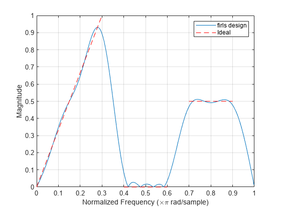
Design a 24th-order antisymmetric filter with piecewise linear passbands.

F = [0 0.3 0.4 0.6 0.7 0.9]; 
A = [0 1.0 0.0 0.0 0.5 0.5];
b = firls(24,F,A,'hilbert');

Plot the desired and actual frequency responses.

[H,f] = freqz(b,1,512,2);
plot(f,abs(H))
hold on
for i = 1:2:6, 
   plot([F(i) F(i+1)],[A(i) A(i+1)],'r--')
end
legend('firls design','Ideal')
grid on
xlabel('Normalized Frequency (\times\pi rad/sample)')
ylabel('Magnitude')

Figure contains an axes object. The axes object with xlabel Normalized Frequency ( times pi blank rad/sample), ylabel Magnitude contains 4 objects of type line. These objects represent firls design, Ideal.

Design an FIR lowpass filter. The passband ranges from DC to 0.45π rad/sample. The stopband ranges from 0.55π rad/sample to the Nyquist frequency. Produce three different designs, changing the weights of the bands in the least-squares fit.

In the first design, make the stopband weight higher than the passband weight by a factor of 100. Use this specification when it is critical that the magnitude response in the stopband is flat and close to 0. The passband ripple is about 100 times higher than the stopband ripple.

bhi = firls(18,[0 0.45 0.55 1],[1 1 0 0],[1 100]);

In the second design, reverse the weights so that the passband weight is 100 times the stopband weight. Use this specification when it is critical that the magnitude response in the passband is flat and close to 1. The stopband ripple is about 100 times higher than the passband ripple.

blo = firls(18,[0 0.45 0.55 1],[1 1 0 0],[100 1]);

In the third design, give the same weight to both bands. The result is a filter with similar ripple in the passband and the stopband.

b = firls(18,[0 0.45 0.55 1],[1 1 0 0],[1 1]);

Visualize the magnitude responses of the three filters.

zerophase(bhi,1)
hold on
zerophase(blo,1)
zerophase(b,1)
hold off
ylim([-.2 1.2])
legend(["bhi: w = [1 100]" "blo: w = [100 1]" "b: w = [1 1]"])

Figure contains an axes object. The axes object with title Zero-Phase Response, xlabel Normalized Frequency ( times pi blank rad/sample), ylabel Amplitude contains 3 objects of type line. These objects represent bhi: w = [1 100], blo: w = [100 1], b: w = [1 1].

Input Arguments

collapse all

Filter order, specified as a real positive scalar.

Normalized frequency points, specified as a real-valued vector. The argument must be in the range [0, 1] , where 1 corresponds to the Nyquist frequency. The number of elements in the vector is always a multiple of 2. The frequencies must be in nondecreasing order.

Desired amplitudes at the points specified in f, specified as a vector. f and a must be the same length. The length must be an even number.

  • The desired amplitude at frequencies between pairs of points (f(k), f(k+1)) for k odd is the line segment connecting the points (f(k), a(k)) and (f(k+1), a(k+1)).

  • The desired amplitude at frequencies between pairs of points (f(k), f(k+1)) for k even is unspecified. The areas between such points are transition regions or regions that are not important for a particular application.

Weights used to adjust the fit in each frequency band, specified as a real-valued vector. The length of w is half the length of f and a, so there is exactly one weight per band.

Filter type for linear-phase filters with odd symmetry (type III and type IV), specified as either 'hilbert' or 'differentiator':

  • 'hilbert' — The output coefficients in b obey the relation b(k) = –b(n + 2 – k), k = 1, ..., n + 1. This class of filters includes the Hilbert transformer, which has a desired amplitude of 1 across the entire band.

  • 'differentiator' — For nonzero amplitude bands, the filter weighs the error by a factor of 1/f2 so that the error at low frequencies is much smaller than at high frequencies. For FIR differentiators, which have an amplitude characteristic proportional to frequency, these filters minimize the maximum relative error (the maximum of the ratio of the error to the desired amplitude).

Output Arguments

collapse all

Filter coefficients, returned as a row vector of length n + 1. The coefficients are in increasing order.

More About

collapse all

Filter Length and Transition Width Incompatibility

If you design a filter such that the product of the filter length and the transition width is large, you might get this warning message: Matrix is close to singular or badly scaled. The following example illustrates this limitation.

b = firls(100,[0 0.15 0.85 1],[1 1 0 0]);
Warning: Matrix is close to singular or badly scaled. Results may be inaccurate. RCOND =  3.056853e-18.
freqz(b,1)

Figure contains 2 axes objects. Axes object 1 with title Phase, xlabel Normalized Frequency (\times\pi rad/sample), ylabel Phase (degrees) contains an object of type line. Axes object 2 with title Magnitude, xlabel Normalized Frequency (\times\pi rad/sample), ylabel Magnitude (dB) contains an object of type line.

In this case, the filter coefficients b might not represent the desired filter. You can check the filter by looking at its frequency response.

Algorithms

firls designs a linear-phase FIR filter that minimizes the weighted integrated squared error between an ideal piecewise linear function and the magnitude response of the filter over a set of desired frequency bands.

Reference [2] describes the theoretical approach behind firls. The function solves a system of linear equations using the MATLAB® \ operator. For a filter of order n, the solution of the equation system involves an inner-product square matrix of size L, where L = (n–1)/2 + 1 when n is odd, and L = n/2 + 1 when n is even.

The input arguments f and a specify the frequency-amplitude characteristics of the filter:

  • f is a vector of pairs of frequency points, specified in the range 0 to 1, where 1 corresponds to the Nyquist frequency. The frequencies must be in increasing order. You can specify duplicate frequency points.

  • a is a vector containing the desired amplitudes at the points specified in f.

    The desired amplitude function at frequencies between pairs of points (f(k), f(k+1)) for k odd is the line segment connecting the points (f(k), a(k)) and (f(k+1), a(k+1)).

    The desired amplitude function at frequencies between pairs of points (f(k), f(k+1)) for k even is unspecified. These are transition ("don’t care") regions.

  • f and a are the same length. This length must be an even number.

This figure illustrates the relationship between the vectors f and a in defining a desired amplitude response.
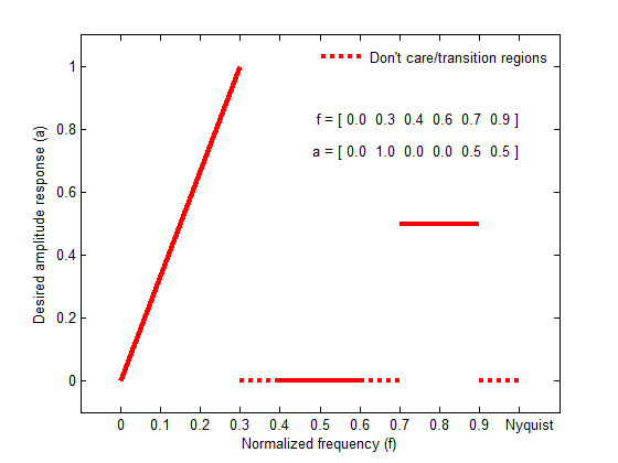
Desired amplitude response vs. normalized frequency. The plot includes the don't-care and transition regions.

The firls function designs type I, II, III, and IV linear-phase filters. Type I and II are the default filters when n is even and odd, respectively, while the 'hilbert' and 'differentiator' flags produce type III (n is even) and IV (n is odd) filters. The various filter types have different symmetries and constraints on their frequency responses (see [1] for details).

Linear Phase Filter TypeFilter OrderSymmetry of CoefficientsResponse H(f), f = 0Response H(f), f = 1 (Nyquist)

Type I

Even

b(k)=b(n+2k),k=1,...,n+1

No restriction

No restriction

Type II

Odd

b(k)=b(n+2k),k=1,...,n+1

No restriction

H(1) = 0

Type III

Even

b(k)=b(n+2k),k=1,...,n+1

H(0) = 0

H(1) = 0

Type IV

Odd

b(k)=b(n+2k),k=1,...,n+1

H(0) = 0

No restriction

References

[1] Oppenheim, Alan V., and Ronald W. Schafer, with John R. Buck. Discrete-Time Signal Processing. Upper Saddle River, NJ: Prentice Hall, 1999.

[2] Parks, Thomas W., and C. Sidney Burrus. Digital Filter Design. Hoboken, NJ: John Wiley & Sons, 1987, pp. 54–83.

Extended Capabilities

C/C++ Code Generation
Generate C and C++ code using MATLAB® Coder™.

Version History

Introduced before R2006a

expand all

Go to top of page