lowpass

Lowpass-filter signals

Syntax

y = lowpass(x,wpass)

y = lowpass(x,fpass,fs)

y = lowpass(xt,fpass)

y = lowpass(___,Name=Value)

[y,d] = lowpass(___)

lowpass(___)

Description

y = lowpass(x,wpass) filters the input signal x using a lowpass filter with normalized passband frequency wpass in units of π rad/sample. lowpass uses a minimum-order filter with a stopband attenuation of 60 dB and compensates for the delay introduced by the filter. If x is a matrix, the function filters each column independently.

y = lowpass(x,fpass,fs) specifies that x has been sampled at a rate of fs hertz. fpass is the passband frequency of the filter in hertz.

y = lowpass(xt,fpass) lowpass-filters the data in timetable xt using a filter with a passband frequency of fpass hertz. The function independently filters all variables in the timetable and all columns inside each variable.

y = lowpass(___,Name=Value) specifies additional options for any of the previous syntaxes using name-value arguments. You can change the stopband attenuation, the Lowpass Filter Steepness, and the type of impulse response of the filter.

[y,d] = lowpass(___) also returns the digitalFilter object d used to filter the input.

lowpass(___) with no output arguments plots the input signal and overlays the filtered signal.

Examples

Lowpass Filtering of Tones

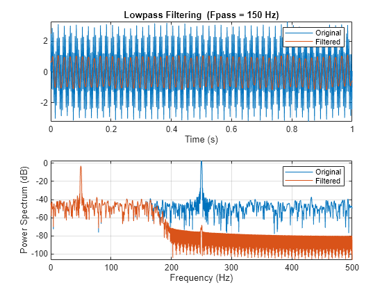
Create a signal sampled at 1 kHz for 1 second. The signal contains two tones, one at 50 Hz and the other at 250 Hz, embedded in Gaussian white noise of variance 1/100. The high-frequency tone has twice the amplitude of the low-frequency tone.

fs = 1e3;
t = 0:1/fs:1;

x = [1 2]*sin(2*pi*[50 250]'.*t) + randn(size(t))/10;

Lowpass-filter the signal to remove the high-frequency tone. Specify a passband frequency of 150 Hz. Display the original and filtered signals, and also their spectra.

lowpass(x,150,fs)

Lowpass Filtering of Musical Signal

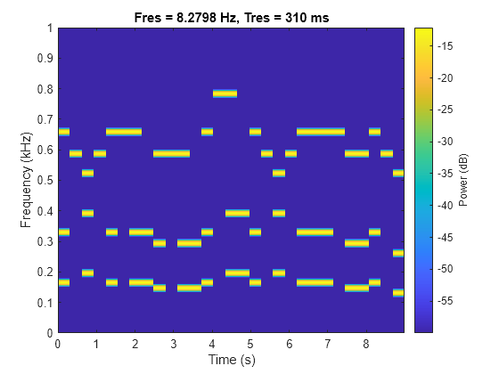
Implement a basic digital music synthesizer and use it to play a traditional song. Specify a sample rate of 2 kHz. Plot the spectrogram of the song.

fs = 2e3;
t = 0:1/fs:0.3-1/fs; fq = [-Inf -9:2]/12;
note = @(f,g) [1 1 1]*sin(2*pi*440*2.^[fq(g)-1 fq(g) fq(f)+1]'.*t);

mel = [5 3 1 3 5 5 5 0 3 3 3 0 5 8 8 0 5 3 1 3 5 5 5 5 3 3 5 3 1]+1;
acc = [5 0 8 0 5 0 5 5 3 0 3 3 5 0 8 8 5 0 8 0 5 5 5 0 3 3 5 0 1]+1;

song = [];
for kj = 1:length(mel)
    song = [song note(mel(kj),acc(kj)) zeros(1,0.01*fs)];
end
song = song/(max(abs(song))+0.1);

% To hear, type sound(song,fs)

pspectrum(song,fs,"spectrogram",TimeResolution=0.31, ...
    OverlapPercent=0,MinThreshold=-60)

Lowpass-filter the signal to separate the melody from the accompaniment. Specify a passband frequency of 450 Hz. Plot the original and filtered signals in the time and frequency domains.

long = lowpass(song,450,fs);

% To hear, type sound(long,fs)

lowpass(song,450,fs)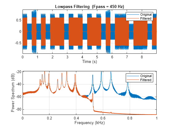

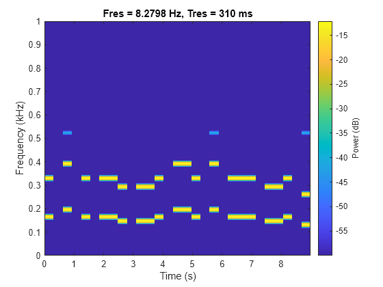
Plot the spectrogram of the accompaniment.

figure
pspectrum(long,fs,"spectrogram",TimeResolution=0.31, ...
    OverlapPercent=0,MinThreshold=-60)

Lowpass Filter Steepness

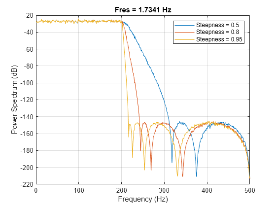
Filter white noise sampled at 1 kHz using an infinite impulse response lowpass filter with a passband frequency of 200 Hz. Use different steepness values. Plot the spectra of the filtered signals.

fs = 1000;
x = randn(20000,1);

[y1,d1] = lowpass(x,200,fs,ImpulseResponse="iir",Steepness=0.5);
[y2,d2] = lowpass(x,200,fs,ImpulseResponse="iir",Steepness=0.8);
[y3,d3] = lowpass(x,200,fs,ImpulseResponse="iir",Steepness=0.95);

pspectrum([y1 y2 y3],fs)
legend("Steepness = " + [0.5 0.8 0.95])

Compute and plot the frequency responses of the filters.

[h1,f] = freqz(d1,1024,fs);
[h2,~] = freqz(d2,1024,fs);
[h3,~] = freqz(d3,1024,fs);

plot(f,mag2db(abs([h1 h2 h3])))
legend("Steepness = " + [0.5 0.8 0.95])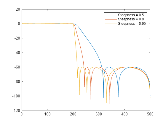

Input Arguments

x — Input signal

vector | matrix

Input signal, specified as a vector or matrix.

Example: sin(2*pi*(0:127)/16)+randn(1,128)/100 specifies a noisy sinusoid

Example: [2 1].*sin(2*pi*(0:127)'./[16 64]) specifies a two-channel sinusoid.

Data Types: single | double
Complex Number Support: Yes

wpass — Normalized passband frequency

scalar in (0, 1)

Normalized passband frequency, specified as a scalar in the interval (0, 1).

fpass — Passband frequency

scalar in (0, fs/2)

Passband frequency, specified as a scalar in the interval (0, fs/2).

fs — Sample rate

positive real scalar

Sample rate, specified as a positive real scalar.

xt — Input timetable

timetable

Input timetable. xt must contain increasing, finite, and equally spaced row times of type duration in seconds.

If a timetable has missing or duplicate time points, you can fix it using the tips in Clean Timetable with Missing, Duplicate, or Nonuniform Times.

Example: timetable(seconds(0:4)',randn(5,1),randn(5,2)) contains a single-channel random signal and a two-channel random signal, sampled at 1 Hz for 4 seconds.

Example: timetable(randn(5,1),randn(5,2),SampleRate=1) contains a single-channel random signal and a two-channel random signal, sampled at 1 Hz for 4 seconds.

Name-Value Arguments

Specify optional pairs of arguments as Name1=Value1,...,NameN=ValueN, where Name is the argument name and Value is the corresponding value. Name-value arguments must appear after other arguments, but the order of the pairs does not matter.

Example: ImpulseResponse="iir",StopbandAttenuation=30 filters the input using a minimum-order IIR filter that attenuates frequencies higher than fpass by 30 dB.

Before R2021a, use commas to separate each name and value, and enclose Name in quotes.

Example: 'ImpulseResponse','iir','StopbandAttenuation',30 filters the input using a minimum-order IIR filter that attenuates frequencies higher than fpass by 30 dB.

ImpulseResponse — Type of impulse response

"auto" (default) | "fir" | "iir"

Type of impulse response of the filter, specified as "fir", "iir", or "auto".

• "fir" — The function designs a minimum-order, linear-phase, finite impulse response (FIR) filter. To compensate for the delay, the function appends to the input signal N/2 zeros, where N is the filter order. The function then filters the signal and removes the first N/2 samples of the output.

  In this case, the input signal must be at least twice as long as the filter that meets the specifications.

• "iir" — The function designs a minimum-order infinite impulse response (IIR) filter and uses the filtfilt function to perform zero-phase filtering and compensate for the filter delay.

  If the signal is not at least three times as long as the filter that meets the specifications, the function designs a filter with smaller order and thus smaller steepness.

• "auto" — The function designs a minimum-order FIR filter if the input signal is long enough, and a minimum-order IIR filter otherwise. Specifically, the function follows these steps:

  • Compute the minimum order that an FIR filter must have to meet the specifications. If the signal is at least twice as long as the required filter order, design and use that filter.

  • If the signal is not long enough, compute the minimum order that an IIR filter must have to meet the specifications. If the signal is at least three times as long as the required filter order, design and use that filter.

  • If the signal is not long enough, truncate the order to one-third the signal length and design an IIR filter of that order. The reduction in order comes at the expense of transition band steepness.

  • Filter the signal and compensate for the delay.

Steepness — Transition band steepness

0.85 (default) | scalar in the interval [0.5, 1)

Transition band steepness, specified as a scalar in the interval [0.5, 1). As the steepness increases, the filter response approaches the ideal lowpass response, but the resulting filter length and the computational cost of the filtering operation also increase. See Lowpass Filter Steepness for more information.

StopbandAttenuation — Filter stopband attenuation

60 (default) | positive scalar in dB

Filter stopband attenuation, specified as a positive scalar in dB.

Output Arguments

y — Filtered signal

vector | matrix | timetable

Filtered signal, returned as a vector, a matrix, or a timetable with the same dimensions as the input.

d — Lowpass filter

digitalFilter object

Lowpass filter used in the filtering operation, returned as a digitalFilter object.

• Use filter(d,x) to filter a signal x using d. Unlike lowpass, the filter function does not compensate for filter delay. You can also use the filtfilt and fftfilt functions with digitalFilter objects.

• Use FVTool to visualize the filter response.

• Use designfilt to edit or generate a digital filter based on frequency-response specifications.

More About

Lowpass Filter Steepness

The Steepness argument controls the width of a filter's transition region. The lower the steepness, the wider the transition region. The higher the steepness, the narrower the transition region.

To interpret the filter steepness, consider the following definitions:

• The Nyquist frequency, f_Nyquist, is the highest frequency component of a signal that can be sampled at a given rate without aliasing. f_Nyquist is 1 (×π rad/sample) when the input signal has no time information, and fs/2 hertz when the input signal is a timetable or when you specify a sample rate.

• The stopband frequency of the filter, f_stop, is the frequency beyond which the attenuation is equal to or greater than the value specified using StopbandAttenuation.

• The transition width of the filter, W, is f_stop – fpass, where fpass is the specified passband frequency.

• Most nonideal filters also attenuate the input signal across the passband. The maximum value of this frequency-dependent attenuation is called the passband ripple. Every filter used by lowpass has a passband ripple of 0.1 dB.

When you specify a value, s, for Steepness, the function computes the transition width as

W = (1 – s) × (f_Nyquist – fpass).

• When Steepness is equal to 0.5, the transition width is 50% of (f_Nyquist – fpass).

• As Steepness approaches 1, the transition width becomes progressively narrower until it reaches a minimum value of 1% of (f_Nyquist – fpass).

• The default value of Steepness is 0.85, which corresponds to a transition width that is 15% of (f_Nyquist – fpass).

Version History

Introduced in R2018a