butter
Butterworth filter design
Syntax
Description
[
designs a lowpass, highpass, bandpass, or bandstop digital Butterworth filter,
depending on the value of b,a] = butter(n,Wn,ftype)ftype and the number of elements
of Wn. The resulting bandpass and bandstop filter designs
are of order 2n.
Note
You might encounter numerical instabilities when designing IIR filters with transfer functions for orders as low as 4. See Transfer Functions and CTF for more information about numerical issues that affect forming the transfer function.
[
designs a digital Butterworth filter and returns its zeros, poles, and gain.
This syntax can include any of the input arguments in previous syntaxes.z,p,k] = butter(___)
[___] = butter(___,"s") designs
an analog Butterworth filter using any of the input or output arguments in
previous syntaxes.
[
designs a lowpass digital Butterworth filter using second-order Cascaded Transfer Functions
(CTF). The function returns matrices that list the denominator and numerator
polynomial coefficients of the filter transfer function, represented as a
cascade of filter sections. This approach generates IIR filters with improved
numerical stability compared to single-section transfer functions. (since R2024b)B,A] = butter(n,Wn,"ctf")
[___] = butter(
designs a lowpass, highpass, bandpass, or bandstop digital Butterworth filter,
and returns the filter representation using the CTF format. The resulting design
sections are of order 2 (lowpass and highpass filters) or 4 (bandpass and
bandstop filters). (since R2024b)n,Wn,ftype,"ctf")
[___,
also returns the overall gain of the system. You must specify
gS] = butter(___)"ctf" to return gS. (since R2024b)
Examples
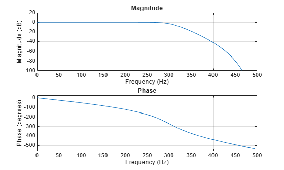
Design a 6th-order lowpass Butterworth filter with a cutoff frequency of 300 Hz, which, for data sampled at 1000 Hz, corresponds to rad/sample. Plot its magnitude and phase responses. Use it to filter a 1000-sample random signal.
fc = 300;
fs = 1000;

[b,a] = butter(6,fc/(fs/2));

freqz(b,a,[],fs)

subplot(2,1,1)
ylim([-100 20])
dataIn = randn(1000,1);
dataOut = filter(b,a,dataIn);
Design a 6th-order Butterworth bandstop filter with normalized edge frequencies of and rad/sample. Plot its magnitude and phase responses. Use it to filter random data.
[b,a] = butter(3,[0.2 0.6],'stop');
freqz(b,a)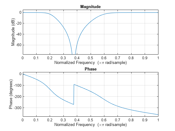
dataIn = randn(1000,1);
dataOut = filter(b,a,dataIn);
Design a 9th-order highpass Butterworth filter. Specify a cutoff frequency of 300 Hz, which, for data sampled at 1000 Hz, corresponds to rad/sample. Plot the magnitude and phase responses. Convert the zeros, poles, and gain to second-order sections. Display the frequency response of the filter.
[z,p,k] = butter(9,300/500,"high");
sos = zp2sos(z,p,k);
freqz(sos)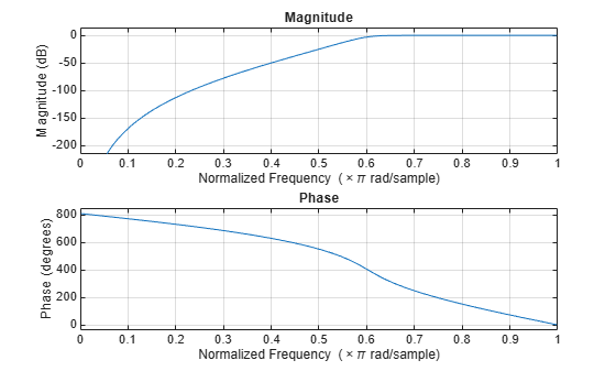
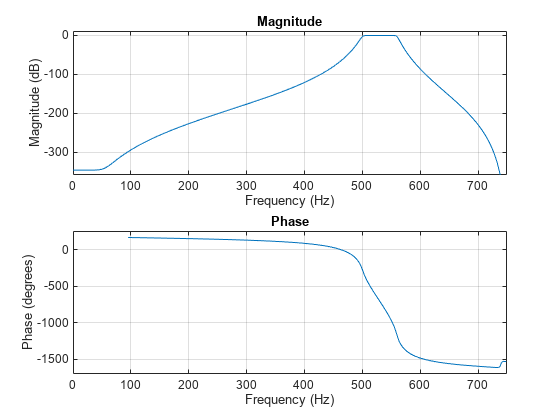
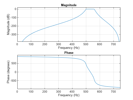
Design a 20th-order Butterworth bandpass filter with a lower cutoff frequency of 500 Hz and a higher cutoff frequency of 560 Hz. Specify a sample rate of 1500 Hz. Use the state-space representation. Convert the state-space representation to second-order sections. Visualize the frequency responses.
fs = 1500;
[A,B,C,D] = butter(10,[500 560]/(fs/2));
sos = ss2sos(A,B,C,D);
freqz(sos,[],fs)
Design an identical filter using designfilt. Visualize the frequency responses.
d = designfilt("bandpassiir",FilterOrder=20, ...
    HalfPowerFrequency1=500,HalfPowerFrequency2=560, ...
    SampleRate=fs);
freqz(d,[],fs)
Design a fifth-order analog Butterworth lowpass filter with a cutoff frequency of 2 GHz. Multiply by to convert the frequency to radians per second. Compute the frequency response of the filter at 4096 points.
n = 5;
wn = 2*pi*2e9;
w = 2*pi*1e9*logspace(-2,1,4096)';

[zb,pb,kb] = butter(n,wn,"s");
[bb,ab] = zp2tf(zb,pb,kb);
[hb,wb] = freqs(bb,ab,w);
gdb = -diff(unwrap(angle(hb)))./diff(wb);
Design a fifth-order Chebyshev Type I filter with a passband edge frequency of 2 GHz and 3 dB of passband ripple. Compute its frequency response.
wp = wn;

[z1,p1,k1] = cheby1(n,3,wp,"s");
[b1,a1] = zp2tf(z1,p1,k1);
[h1,w1] = freqs(b1,a1,w);
gd1 = -diff(unwrap(angle(h1)))./diff(w1);
Design a fifth-order Chebyshev Type II filter with a stopband edge frequency of 2.5 GHz and 30 dB of stopband attenuation. Compute its frequency response.
ws = 2*pi*2.5e9;

[z2,p2,k2] = cheby2(n,30,ws,"s");
[b2,a2] = zp2tf(z2,p2,k2);
[h2,w2] = freqs(b2,a2,w);
gd2 = -diff(unwrap(angle(h2)))./diff(w2);
Design a fifth-order elliptic filter with the same passband and stopband edge frequencies, 3 dB of passband ripple, and 30 dB of stopband attenuation. Compute its frequency response.
[ze,pe,ke] = ellip(n,3,30,wp,"s");
[be,ae] = zp2tf(ze,pe,ke);
[he,we] = freqs(be,ae,w);
gde = -diff(unwrap(angle(he)))./diff(we);
Design a fifth-order Bessel filter with the same edge frequency. Compute its frequency response.
[zf,pf,kf] = besself(n,wn);
[bf,af] = zp2tf(zf,pf,kf);
[hf,wf] = freqs(bf,af,w);
gdf = -diff(unwrap(angle(hf)))./diff(wf);
Plot the attenuation in decibels. Express the frequency in gigahertz. Compare the filters.
fGHz = [wb w1 w2 we wf]/(2e9*pi);
plot(fGHz,mag2db(abs([hb h1 h2 he hf])))
axis([0 5 -45 5])
grid on
xlabel("Frequency (GHz)")
ylabel("Attenuation (dB)")
legend(["butter" "cheby1" "cheby2" "ellip" "besself"], ...
    Location="southwest")
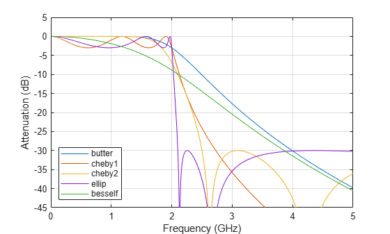
The Butterworth and Chebyshev Type II filters have flat passbands and wide transition bands. The Chebyshev Type I and elliptic filters roll off faster but have passband ripple. The frequency input to the Chebyshev Type II design function sets the beginning of the stopband rather than the end of the passband. Elliptic filters offer steeper rolloff characteristics than Butterworth and Chebyshev filters, but they are equiripple in both the passband and the stopband. Of these four classical filter types, elliptic filters usually meet a given set of filter performance specifications with the lowest filter order.
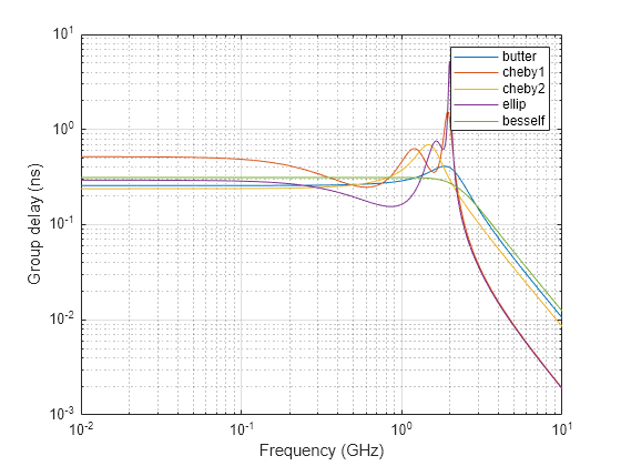
Plot the group delay in samples. Express the frequency in gigahertz and the group delay in nanoseconds. Compare the filters. The Bessel filter has approximately constant group delay along the passband.
gdns = [gdb gd1 gd2 gde gdf]*1e9;
gdns(gdns<0) = NaN;
loglog(fGHz(2:end,:),gdns)
grid on
xlabel("Frequency (GHz)")
ylabel("Group delay (ns)")
legend(["butter" "cheby1" "cheby2" "ellip" "besself"], ...
    Location="southwest")
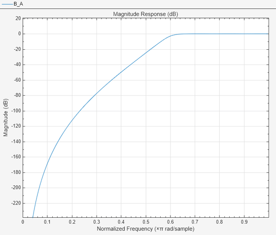
Design a ninth-order highpass Butterworth filter with a cutoff frequency of 300 Hz and sampling rate of 1000 Hz. Return the coefficients of the filter system as a cascade of second-order sections.
Wn = 300/(1000/2);
[B,A] = butter(9,Wn,"high","ctf")
B = 5×3

    0.2544   -0.2544         0
    0.2544   -0.5088    0.2544
    0.2544   -0.5088    0.2544
    0.2544   -0.5088    0.2544
    0.2544   -0.5088    0.2544
A = 5×3

    1.0000    0.1584         0
    1.0000    0.3264    0.0561
    1.0000    0.3575    0.1570
    1.0000    0.4189    0.3554
    1.0000    0.5304    0.7165
Plot the magnitude response of the filter.
filterAnalyzer(B,A)
Input Arguments
Output Arguments
More About
Numerical Instability of Transfer Function Syntax
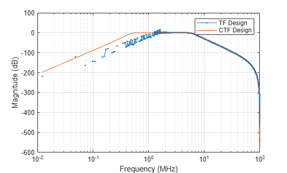
In general, use cascaded transfer functions ("ctf" syntaxes) to design IIR digital filters. If you design the filter using transfer functions (any of the [b,a] syntaxes), you might encounter numerical instabilities. These instabilities are due to round-off errors and can occur for an order n as low as 4. This example illustrates this limitation.
n = 6;
Fs = 200e6;
Wn = [0.5e6 6e6]/(Fs/2);
ftype = "bandpass";

% Transfer Function (TF) design
[b,a] = butter(n,Wn,ftype);    % This is an unstable filter

% CTF design
[B,A] = butter(n,Wn,ftype,"ctf");

% Compare frequency responses
[hTF,f] = freqz(b,a,8192,Fs);
hCTF = freqz(B,A,8192,Fs);

semilogx(f/1e6,db(hTF),".-",f/1e6,db(hCTF))
grid on
legend(["TF Design" "CTF Design"])
xlabel("Frequency (MHz)")
ylabel("Magnitude (dB)")
Algorithms
Butterworth filters have a magnitude response that is maximally flat in the passband and monotonic overall. This smoothness comes at the price of decreased rolloff steepness. Elliptic and Chebyshev filters generally provide steeper rolloff for a given filter order.
butter uses a five-step algorithm:
It finds the lowpass analog prototype poles, zeros, and gain using the function
buttap.It converts the poles, zeros, and gain into state-space form.
If required, it uses a state-space transformation to convert the lowpass filter into a bandpass, highpass, or bandstop filter with the desired frequency constraints.
For digital filter design, it uses
bilinearto convert the analog filter into a digital filter through a bilinear transformation with frequency prewarping. Careful frequency adjustment enables the analog filters and the digital filters to have the same frequency response magnitude atWnor atw1andw2.It converts the state-space filter back to its transfer function or zero-pole-gain form, as required.
References
[1] Lyons, Richard G. Understanding Digital Signal Processing. Upper Saddle River, NJ: Prentice Hall, 2004.