Main Content

cheby2

Chebyshev Type II filter design

Description

example

[b,a] = cheby2(n,Rs,Ws) returns the transfer function coefficients of an nth-order lowpass digital Chebyshev Type II filter with normalized stopband edge frequency Ws and Rs decibels of stopband attenuation down from the peak passband value.

example

[b,a] = cheby2(n,Rs,Ws,ftype) designs a lowpass, highpass, bandpass, or bandstop Chebyshev Type II filter, depending on the value of ftype and the number of elements of Ws. The resulting bandpass and bandstop designs are of order 2n.

Note:   See Limitations for information about numerical issues that affect forming the transfer function.

example

[z,p,k] = cheby2(___) designs a lowpass, highpass, bandpass, or bandstop digital Chebyshev Type II filter and returns its zeros, poles, and gain. This syntax can include any of the input arguments in previous syntaxes.

example

[A,B,C,D] = cheby2(___) designs a lowpass, highpass, bandpass, or bandstop digital Chebyshev Type II filter and returns the matrices that specify its state-space representation.

example

[___] = cheby2(___,'s') designs a lowpass, highpass, bandpass, or bandstop analog Chebyshev Type II filter with stopband edge angular frequency Ws and Rs decibels of stopband attenuation.

Examples

collapse all

Design a 6th-order lowpass Chebyshev Type II filter with 50 dB of stopband attenuation and a stopband edge frequency of 300 Hz, which, for data sampled at 1000 Hz, corresponds to 0.6π rad/sample. Plot its magnitude and phase responses. Use it to filter a 1000-sample random signal.

fc = 300;
fs = 1000;

[b,a] = cheby2(6,50,fc/(fs/2));

freqz(b,a,[],fs)

subplot(2,1,1)
ylim([-100 20])

Figure contains 2 axes objects. Axes object 1 with title Phase, xlabel Frequency (Hz), ylabel Phase (degrees) contains an object of type line. Axes object 2 with title Magnitude, xlabel Frequency (Hz), ylabel Magnitude (dB) contains an object of type line.

dataIn = randn(1000,1);
dataOut = filter(b,a,dataIn);

Design a 6th-order Chebyshev Type II bandstop filter with normalized edge frequencies of 0.2π and 0.6π rad/sample and 50 dB of stopband attenuation. Plot its magnitude and phase responses. Use it to filter random data.

[b,a] = cheby2(3,50,[0.2 0.6],'stop');
freqz(b,a)

Figure contains 2 axes objects. Axes object 1 with title Phase, xlabel Normalized Frequency (\times\pi rad/sample), ylabel Phase (degrees) contains an object of type line. Axes object 2 with title Magnitude, xlabel Normalized Frequency (\times\pi rad/sample), ylabel Magnitude (dB) contains an object of type line.

dataIn = randn(1000,1);
dataOut = filter(b,a,dataIn);

Design a 9th-order highpass Chebyshev Type II filter with 20 dB of stopband attenuation and a stopband edge frequency of 300 Hz, which, for data sampled at 1000 Hz, corresponds to 0.6π rad/sample. Plot the magnitude and phase responses. Convert the zeros, poles, and gain to second-order sections for use by fvtool.

[z,p,k] = cheby2(9,20,300/500,'high');
sos = zp2sos(z,p,k);
fvtool(sos,'Analysis','freq')

Figure Figure 1: Magnitude Response (dB) and Phase Response contains an axes object. The axes object with title Magnitude Response (dB) and Phase Response, xlabel Normalized Frequency ( times pi blank rad/sample), ylabel Magnitude (dB) contains an object of type line.

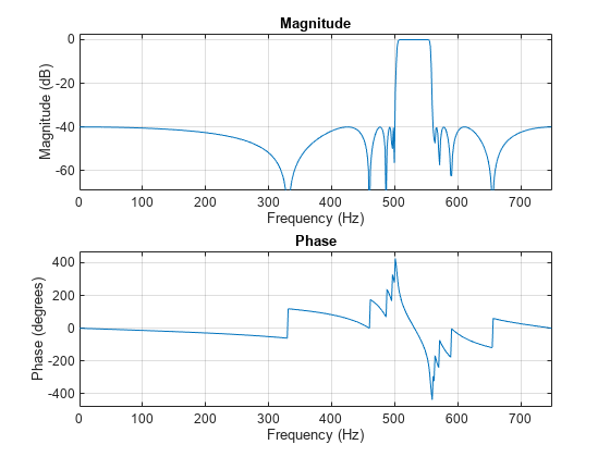
Design a 20th-order Chebyshev Type II bandpass filter with a lower stopband frequency of 500 Hz and a higher stopband frequency of 560 Hz. Specify a stopband attenuation of 40 dB and a sample rate of 1500 Hz. Use the state-space representation. Design an identical filter using designfilt.

[A,B,C,D] = cheby2(10,40,[500 560]/750);
d = designfilt('bandpassiir','FilterOrder',20, ...
    'StopbandFrequency1',500,'StopbandFrequency2',560, ...
    'StopbandAttenuation',40,'SampleRate',1500);

Convert the state-space representation to second-order sections. Visualize the frequency responses using fvtool.

sos = ss2sos(A,B,C,D);
fvt = fvtool(sos,d,'Fs',1500);
legend(fvt,'cheby2','designfilt')

Figure Figure 1: Magnitude Response (dB) contains an axes object. The axes object with title Magnitude Response (dB), xlabel Frequency (Hz), ylabel Magnitude (dB) contains 2 objects of type line. These objects represent cheby2, designfilt.

Design a 5th-order analog Butterworth lowpass filter with a cutoff frequency of 2 GHz. Multiply by 2π to convert the frequency to radians per second. Compute the frequency response of the filter at 4096 points.

n = 5;
fc = 2e9;

[zb,pb,kb] = butter(n,2*pi*fc,"s");
[bb,ab] = zp2tf(zb,pb,kb);
[hb,wb] = freqs(bb,ab,4096);

Design a 5th-order Chebyshev Type I filter with the same edge frequency and 3 dB of passband ripple. Compute its frequency response.

[z1,p1,k1] = cheby1(n,3,2*pi*fc,"s");
[b1,a1] = zp2tf(z1,p1,k1);
[h1,w1] = freqs(b1,a1,4096);

Design a 5th-order Chebyshev Type II filter with the same edge frequency and 30 dB of stopband attenuation. Compute its frequency response.

[z2,p2,k2] = cheby2(n,30,2*pi*fc,"s");
[b2,a2] = zp2tf(z2,p2,k2);
[h2,w2] = freqs(b2,a2,4096);

Design a 5th-order elliptic filter with the same edge frequency, 3 dB of passband ripple, and 30 dB of stopband attenuation. Compute its frequency response.

[ze,pe,ke] = ellip(n,3,30,2*pi*fc,"s");
[be,ae] = zp2tf(ze,pe,ke);
[he,we] = freqs(be,ae,4096);

Design a 5th-order Bessel filter with the same edge frequency. Compute its frequency response.

[zf,pf,kf] = besself(n,2*pi*fc);
[bf,af] = zp2tf(zf,pf,kf);
[hf,wf] = freqs(bf,af,4096);

Plot the attenuation in decibels. Express the frequency in gigahertz. Compare the filters.

plot([wb w1 w2 we wf]/(2e9*pi), ...
    mag2db(abs([hb h1 h2 he hf])))
axis([0 5 -45 5])
grid
xlabel("Frequency (GHz)")
ylabel("Attenuation (dB)")
legend(["butter" "cheby1" "cheby2" "ellip" "besself"])

Figure contains an axes object. The axes object with xlabel Frequency (GHz), ylabel Attenuation (dB) contains 5 objects of type line. These objects represent butter, cheby1, cheby2, ellip, besself.

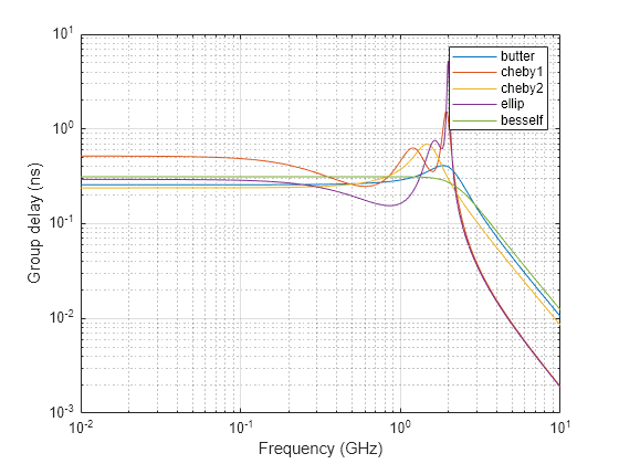
The Butterworth and Chebyshev Type II filters have flat passbands and wide transition bands. The Chebyshev Type I and elliptic filters roll off faster but have passband ripple. The frequency input to the Chebyshev Type II design function sets the beginning of the stopband rather than the end of the passband. The Bessel filter has approximately constant group delay along the passband.

Input Arguments

collapse all

Filter order, specified as an integer scalar. For bandpass and bandstop designs, n represents one-half the filter order.

Data Types: double

Stopband attenuation down from the peak passband value, specified as a positive scalar expressed in decibels.

If your specification, ℓ, is in linear units, you can convert it to decibels using Rs = –20 log10ℓ.

Data Types: double

Stopband edge frequency, specified as a scalar or a two-element vector. The stopband edge frequency is the frequency at which the magnitude response of the filter is Rs decibels. Larger values of stopband attenuation, Rs, result in wider transition bands.

  • If Ws is a scalar, then cheby2 designs a lowpass or highpass filter with edge frequency Ws.

    If Ws is the two-element vector [w1 w2], where w1 < w2, then cheby2 designs a bandpass or bandstop filter with lower edge frequency w1 and higher edge frequency w2.

  • For digital filters, the stopband edge frequencies must lie between 0 and 1, where 1 corresponds to the Nyquist rate—half the sample rate or π rad/sample.

    For analog filters, the stopband edge frequencies must be expressed in radians per second and can take on any positive value.

Data Types: double

Filter type, specified as one of the following:

  • 'low' specifies a lowpass filter with stopband edge frequency Ws. 'low' is the default for scalar Ws.

  • 'high' specifies a highpass filter with stopband edge frequency Ws.

  • 'bandpass' specifies a bandpass filter of order 2n if Ws is a two-element vector. 'bandpass' is the default when Ws has two elements.

  • 'stop' specifies a bandstop filter of order 2n if Ws is a two-element vector.

Output Arguments

collapse all

Transfer function coefficients of the filter, returned as row vectors of length n + 1 for lowpass and highpass filters and 2n + 1 for bandpass and bandstop filters.

  • For digital filters, the transfer function is expressed in terms of b and a as

    H(z)=B(z)A(z)=b(1)+b(2)z1++b(n+1)zna(1)+a(2)z1++a(n+1)zn.

  • For analog filters, the transfer function is expressed in terms of b and a as

    H(s)=B(s)A(s)=b(1)sn+b(2)sn1++b(n+1)a(1)sn+a(2)sn1++a(n+1).

Data Types: double

Zeros, poles, and gain of the filter, returned as two column vectors of length n (2n for bandpass and bandstop designs) and a scalar.

  • For digital filters, the transfer function is expressed in terms of z, p, and k as

    H(z)=k(1z(1)z1)(1z(2)z1)(1z(n)z1)(1p(1)z1)(1p(2)z1)(1p(n)z1).

  • For analog filters, the transfer function is expressed in terms of z, p, and k as

    H(s)=k(sz(1))(sz(2))(sz(n))(sp(1))(sp(2))(sp(n)).

Data Types: double

State-space representation of the filter, returned as matrices. If m = n for lowpass and highpass designs and m = 2n for bandpass and bandstop filters, then A is m × m, B is m × 1, C is 1 × m, and D is 1 × 1.

  • For digital filters, the state-space matrices relate the state vector x, the input u, and the output y through

    x(k+1)=Ax(k)+Bu(k)y(k)=Cx(k)+Du(k).

  • For analog filters, the state-space matrices relate the state vector x, the input u, and the output y through

    x˙=Ax+Buy=Cx+Du.

Data Types: double

More About

collapse all

Limitations

Numerical Instability of Transfer Function Syntax

In general, use the [z,p,k] syntax to design IIR filters. To analyze or implement your filter, you can then use the [z,p,k] output with zp2sos. If you design the filter using the [b,a] syntax, you might encounter numerical problems. These problems are due to round-off errors and can occur for n as low as 4. The following example illustrates this limitation.

n = 6; 
Rs = 80; 
Wn = [2.5e6 29e6]/500e6;
ftype = 'bandpass';

% Transfer function design
[b,a] = cheby2(n,Rs,Wn,ftype);      % This filter is unstable

% Zero-pole-gain design
[z,p,k] = cheby2(n,Rs,Wn,ftype);
sos = zp2sos(z,p,k);

% Plot and compare the results
hfvt = fvtool(b,a,sos,'FrequencyScale','log');
legend(hfvt,'TF Design','ZPK Design')

Figure Figure 1: Magnitude Response (dB) contains an axes object. The axes object with title Magnitude Response (dB), xlabel Normalized Frequency ( times pi blank rad/sample), ylabel Magnitude (dB) contains 2 objects of type line. These objects represent TF Design, ZPK Design.

Algorithms

Chebyshev Type II filters are monotonic in the passband and equiripple in the stopband. Type II filters do not roll off as fast as Type I filters, but are free of passband ripple.

cheby2 uses a five-step algorithm:

  1. It finds the lowpass analog prototype poles, zeros, and gain using the function cheb2ap.

  2. It converts poles, zeros, and gain into state-space form.

  3. If required, it uses a state-space transformation to convert the lowpass filter into a bandpass, highpass, or bandstop filter with the desired frequency constraints.

  4. For digital filter design, it uses bilinear to convert the analog filter into a digital filter through a bilinear transformation with frequency prewarping. Careful frequency adjustment the analog filters and the digital filters to have the same frequency response magnitude at Ws or w1 and w2.

  5. It converts the state-space filter back to transfer function or zero-pole-gain form, as required.

Extended Capabilities

Version History

Introduced before R2006a