showCollisionArray

Show array of collision objects in figure

Since R2023b

Syntax

[ax,patches] = showCollisionArray(collArray)

[___] = showCollisionArray(___,Name=Value)

Description

[ax,patches] = showCollisionArray(collArray) plots a collision object array in a figure and returns the axes that the collision objects are plotted on and the patches of each collision object.

[___] = showCollisionArray(___,Name=Value) specifies additional options using one or more name-value arguments in addition to all arguments from the previous syntax. For example, Parent=ax1 specifies ax1 as the axes in which to draw the collision objects.

Examples

Decompose Non-Convex Meshes for Collision Checking

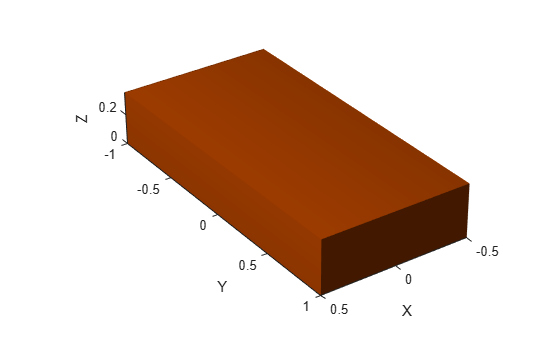
Load an STL file containing a rectangular bin triangulation, and then visualize the bin triangulation.

meshTri = stlread("bin.stl");
trisurf(meshTri)
axis equal

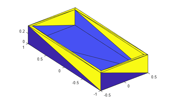
Create a collision mesh using the points from the triangulation of the bin, and then visualize the mesh. Note that, when you approximate the bin triangulation as one collision mesh, the collisionMesh object uses the convex hull of the bin triangulation to approximate the bin. As a result the collision mesh is convex, unlike the non-convex bin triangulation. The collisionMesh object does this because collision checking is most efficient with convex meshes. However, this convex approximation is not ideal for bins because robots can manipulate bins or objects inside of bins.

meshColl = collisionMesh(meshTri.Points);
[~,p] = show(meshColl);
view(145,30) % Change view so it is easier to view the inside of bin
axis equal
hold on

Create a soda can using a collision cylinder, and set the pose such that it sits in the center of the bin. Then, show it in the convex collision mesh.

sodacan = collisionCylinder(0.1,0.4,Pose=trvec2tform([0 0 .3]));
show(sodacan);

Set the box to be transparent so that you can see the overlap between the bin and the soda can.

p.FaceAlpha = 0.25;
hold off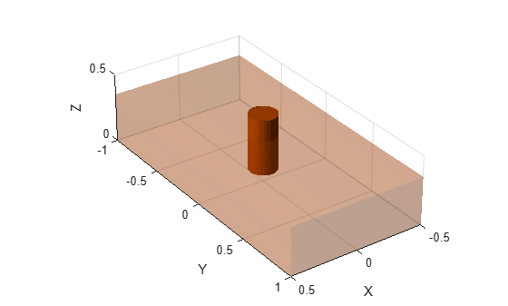

Check collision between the soda can and the convex approximation of the bin, and note that they are in collision.

isCollidingConvex = checkCollision(sodacan,meshColl)

isCollidingConvex = 1

To get a better approximation of the bin for collision checking, decompose the original non-convex mesh into multiple convex meshes using voxelized hierarchical approximate convex decomposition (V-HACD).

Use the collisionVHACD function to decompose the original non-convex triangulation into convex collision meshes. Then, show the decomposed bin with the soda can.

decomposedBin = collisionVHACD(meshTri);
showCollisionArray([decomposedBin {sodacan}]);
view(145,30)
axis equal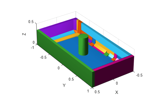

Check collision with all the meshes that approximate the bin. Note that the soda can is not in collision with the decomposed non-convex approximation of the bin. If you require a more accurate decomposition of the bin, you can specify custom solver options using the vhacdOptions object.

isColliding = false(1,length(decomposedBin));
for i = 1:length(decomposedBin)
    isColliding(i) = checkCollision(sodacan,decomposedBin{i});
end
isCollidingAll = all(isColliding)

isCollidingAll = logical
   0

Input Arguments

collArray — Collision objects

N-element cell array of collision geometry objects

Collision objects, specified as an N-element cell array of collision geometry objects. N is the number of collision objects in the cell array. A collision object must be one of these objects:

• collisionBox

• collisionCapsule

• collisionCylinder

• collisionMesh

• collisionSphere

Name-Value Arguments

Specify optional pairs of arguments as Name1=Value1,...,NameN=ValueN, where Name is the argument name and Value is the corresponding value. Name-value arguments must appear after other arguments, but the order of the pairs does not matter.

Example: showCollisionArray(collArr,Parent=ax1) specifies ax1 as the axes in which to draw the collision objects.

Parent — Parent axes

Axes object

Parent axes, specified as an Axes object in which to draw the collision objects in collArray. By default, the function plots the collision objects in the active axes.

ColorOrder — Color order

three-column matrix of RGB triplets

Color order, specified as a three-column matrix of RGB triplets. This property defines the palette of colors MATLAB^® uses to create plot objects such as Line, Scatter, and Bar objects. Each row of the matrix is an RGB triplet. An RGB triplet is a three-element vector whose elements specify the intensities of the red, green, and blue components of a color. The intensities must be in the range [0, 1].

This table lists the default colors.

RGB Triplet	Hexadecimal Color Code	Appearance
[0 0.4470 0.7410]	"#0072BD"
[0.8500 0.3250 0.0980]	"#D95319"
[0.9290 0.6940 0.1250]	"#EDB120"
[0.4940 0.1840 0.5560]	"#7E2F8E"
[0.4660 0.6740 0.1880]	"#77AC30"
[0.3010 0.7450 0.9330]	"#4DBEEE"
[0.6350 0.0780 0.1840]	"#A2142F"

MATLAB assigns colors to objects according to their order of creation. For example, when plotting lines, the first line uses the first color, the second line uses the second color, and so on. If there are more lines than colors, then the cycle repeats.

Changing Color Order Before or After Plotting

You can change the color order in either of these ways:

• Call the colororder function to change the color order for all the axes in a figure. The colors of existing plots in the figure update immediately. If you place additional axes into the figure, those axes also use the new color order. If you continue to call plotting commands, those commands also use the new colors.

• Set the ColorOrder property of the axes, call the hold function to set the axes hold state to "on", and then call the desired plotting functions. Unlike calling the colororder function, this process sets the color order for only the specified axes, not the entire figure. You must set the hold state to "on" to ensure that subsequent plotting commands do not reset the axes to use the default color order.

Output Arguments

ax — Axes graphic handle

Axes object

Axes graphic handle, returned as an Axes object. This object contains the properties of the figure that you plot the collision objects onto.

patches — Patches of collision objects

N-element patch array

Patches of collision objects, returned as N-element patch array corresponding to the collision objects. N is the number of collision objects in the patch array.

Version History

Introduced in R2023b