Detect Image Anomalies Using Pretrained ResNet-18 Feature Embeddings
This example shows how to train a similarity-based anomaly detector using one-class learning of feature embeddings extracted from a pretrained ResNet-18 convolutional neural network.
This example applies patch distribution modeling (PaDiM) [1] to train an anomaly detection classifier. During training, you fit a Gaussian distribution that models the mean and covariance of normal image features. During testing, the classifier labels images whose features deviate from the Gaussian distribution by more than a certain threshold as anomalous. PaDiM is a similarity-based method because the similarity between test images and the normal image distribution drives classification. The PaDiM method has several practical advantages.
PaDiM extracts features from a pretrained CNN without requiring that you retrain the network. Therefore, you can run the example efficiently without special hardware requirements such as a GPU.
PaDiM is a one-class learning approach. The classification model is trained using only normal images. Training does not require images with anomalies, which can be rare, expensive, or unsafe to obtain for certain applications.
PaDiM is an explainable classification method. The PaDiM classifier generates an anomaly score for each spatial patch. You can visualize the scores as a heatmap to localize anomalies and gain insight into the model.
The PaDiM method is suitable for image data sets that can be cropped to match the input size of the pretrained CNN. The input size of the CNN depends on the data used to train the network. For applications requiring more flexibility in image size, an alternative approach might be more appropriate. For an example of such an approach, see Detect Image Anomalies Using Explainable FCDD Network.

Download Concrete Crack Images for Classification Data Set
This example uses the Concrete Crack Images for Classification data set [4] [5]. The data set contains images of two classes: Negative images (or normal images) without cracks present in the road and Positive images (or anomaly images) with cracks. The data set provides 20,000 images of each class. The size of the data set is about 230 MB.
Set dataDir as the desired location of the data set.
dataDir = fullfile(tempdir,"ConcreteCrackDataset");
if ~exist(dataDir,"dir")
    mkdir(dataDir);
end
To download the data set, go to this link: https://data.mendeley.com/datasets/5y9wdsg2zt/2. Extract the ZIP file to obtain a RAR file, then extract the contents of the RAR file into the directory specified by the dataDir variable. When extracted successfully, dataDir contains two subdirectories: Negative and Positive.
Load and Preprocess Data
Create an imageDatastore that reads and manages the image data. Label each image as Positive or Negative according to the name of its directory.
imdsPositive = imageDatastore(fullfile(dataDir,"Positive"),LabelSource="foldernames");
imdsNegative = imageDatastore(fullfile(dataDir,"Negative"),LabelSource="foldernames");
Display an example of each class. Display a negative, or good, image without crack anomalies on the left. In the good image, imperfections and deviations in texture are small. Display a positive, or anomalous, image on the right. The anomalous image shows a large black crack oriented vertically.
samplePositive = preview(imdsPositive);
sampleNegative = preview(imdsNegative);
montage({sampleNegative,samplePositive})
title("Road Images Without (Left) and with (Right) Cracks")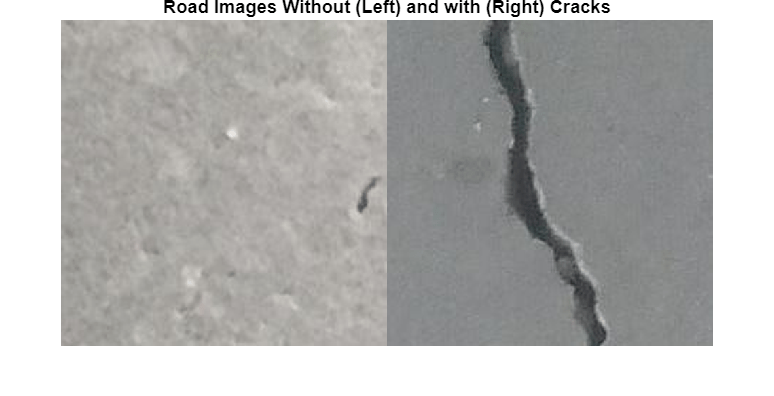
Partition Data into Training, Calibration, and Test Sets
To simulate a more typical semisupervised workflow, create a training set of 250 images from the Negative class only. Allocate 100 Negative images and 100 Positive images to a calibration set. This example uses a calibration set to pick a threshold for the classifier. The classifier labels images with anomaly scores above the threshold as anomalous. Using separate calibration and test sets avoids information leaking from the test set into the design of the classifier. Allocate 1000 Negative images and 1000 Positive images to a test set.
numTrainNormal = 250;
numCal = 100;
numTest = 1000;

[imdsTestPos,imdsCalPos] = splitEachLabel(imdsPositive,numTest,numCal);
[imdsTrainNeg,imdsTestNeg,imdsCalNeg] = splitEachLabel(imdsNegative, ...
    numTrainNormal,numTest,numCal,"randomized");

trainFiles = imdsTrainNeg.Files;
calibrationFiles = cat(1,imdsCalPos.Files,imdsCalNeg.Files);
testFiles = cat(1,imdsTestPos.Files,imdsTestNeg.Files);

imdsTrain = imageDatastore(trainFiles,LabelSource="foldernames");
imdsCal = imageDatastore(calibrationFiles,LabelSource="foldernames");
imdsTest = imageDatastore(testFiles,LabelSource="foldernames");
Define an anonymous function, addLabelFcn, that creates a one-hot encoded representation of label information from an input image. Then, transform the datastores by using the transform function such that the datastores return a cell array of image data and a corresponding one-hot encoded array. The transform function applies the operations specified by addLabelFcn.
addLabelFcn = @(x,info) deal({x,onehotencode(info.Label,1)},info);
tdsTrain = transform(imdsTrain,addLabelFcn,IncludeInfo=true);
tdsCal = transform(imdsCal,addLabelFcn,IncludeInfo=true);
tdsTest = transform(imdsTest,addLabelFcn,IncludeInfo=true);
Resize and Crop Images
Define an anonymous function, resizeAndCropImageFcn, that applies the resizeAndCropForConcreteAnomalyDetector helper function to the input images. The resizeAndCropForConcreteAnomalyDetector helper function resizes and center crops input images, and is attached to the example as a supporting file. Transform the datastores by using the transform function with the operations specified by resizeAndCropImageFcn. This operation crops each image in the training, calibration, and test datastores to a size of 244-by-224 to match the input size of the pretrained CNN.
resizeImageSize = [256 256];
targetImageSize = [224 224];
resizeAndCropImageFcn = @(x,info) ...
    deal({resizeAndCropForConcreteAnomalyDetector(x{1},resizeImageSize,targetImageSize),x{2}});
tdsTrain = transform(tdsTrain,resizeAndCropImageFcn);
tdsCal = transform(tdsCal,resizeAndCropImageFcn);
tdsTest = transform(tdsTest,resizeAndCropImageFcn);
Batch Training Data
Create a minibatchqueue (Deep Learning Toolbox) object that manages the mini-batches of training data. The minibatchqueue object automatically converts data to a dlarray (Deep Learning Toolbox) object that enables automatic differentiation in deep learning applications.
Specify the mini-batch data extraction format as "SSCB" (spatial, spatial, channel, batch).
minibatchSize = 128;
trainQueue = minibatchqueue(tdsTrain, ...
    PartialMiniBatch="return", ...
    MiniBatchFormat=["SSCB","CB"], ...
    MiniBatchSize=minibatchSize);
Create PaDiM Model
This example applies the PaDiM method described in [1]. The basic idea of PaDiM is to simplify 2-D images into a lower resolution grid of embedding vectors that encode features extracted from a subset of layers of a pretrained CNN. Each embedding vector generated from the lower resolution CNN layers corresponds to a spatial patch of pixels in the original resolution image. The training step generates feature embedding vectors for all training set images and fits a statistical Gaussian distribution to the training data. A trained PaDiM classifier model consists of the mean and covariance matrix describing the learned Gaussian distribution for normal training images.
Extract Image Features from Pretrained CNN
This example uses the ResNet-18 network [2] to extract features of input images. ResNet-18 is a convolutional neural network with 18 layers and is pretrained on ImageNet [3].
Extract features from three layers of ResNet-18 located at the end of the first, second, and third blocks. For an input image of size 224-by-224, these layers correspond to activations with spatial resolutions of 56-by-56, 28-by-28, and 14-by-14, respectively. For example, the XTrainFeatures1 variable contains 56-by-56 feature vectors from the bn2b_branch2b layer for each training set image. The layer activations with higher and lower spatial resolutions provide a balance between greater visual detail and global context, respectively.
net = imagePretrainedNetwork("resnet18");

feature1LayerName = "bn2b_branch2b";
feature2LayerName = "bn3b_branch2b";
feature3LayerName = "bn4b_branch2b";

XTrainFeatures1 = [];
XTrainFeatures2 = [];
XTrainFeatures3 = [];

reset(trainQueue);
shuffle(trainQueue);
idx = 1;
while hasdata(trainQueue)
    [X,T] = next(trainQueue);

    XTrainFeatures1 = cat(4,XTrainFeatures1,predict(net,extractdata(X),Outputs=feature1LayerName));
    XTrainFeatures2 = cat(4,XTrainFeatures2,predict(net,extractdata(X),Outputs=feature2LayerName));
    XTrainFeatures3 = cat(4,XTrainFeatures3,predict(net,extractdata(X),Outputs=feature3LayerName));
    idx = idx+size(X,4);
end
Concatenate Feature Embeddings
Combine the features extracted from the three ResNet-18 layers by using the concatenateEmbeddings helper function defined at the end of this example. The concatenateEmbeddings helper function upsamples the feature vectors extracted from the second and third blocks of ResNet-18 to match the spatial resolution of the first block and concatenates the three feature vectors.
XTrainFeatures1 = gather(XTrainFeatures1);
XTrainFeatures2 = gather(XTrainFeatures2);
XTrainFeatures3 = gather(XTrainFeatures3);
XTrainEmbeddings = concatenateEmbeddings(XTrainFeatures1,XTrainFeatures2,XTrainFeatures3);
The variable XTrainEmbeddings is a numeric array containing feature embedding vectors for the training image set. The first two spatial dimensions correspond to the number of spatial patches in each image. The 56-by-56 spatial patches match the size of the bn2b_branch2b layer of ResNet-18. The third dimension corresponds to the channel data, or the length of the feature embedding vector for each patch. The fourth dimension corresponds to the number of training images.
whos XTrainEmbeddingsName Size Bytes Class Attributes XTrainEmbeddings 56x56x448x250 1404928000 single
Randomly Downsample Feature Embedding Channel Dimension
Reduce the dimensionality of the embedding vector by randomly selecting a subset of 100 out of 448 elements in the channel dimension to keep. As shown in [1], this random dimensionality reduction step increases classification efficiency without decreasing accuracy.
selectedChannels = 100;
totalChannels = 448;
rIdx = randi(totalChannels,[1 selectedChannels]);
XTrainEmbeddings = XTrainEmbeddings(:,:,rIdx,:);
Compute Mean and Covariance of Gaussian Distribution
Model the training image patch embedding vectors as a Gaussian distribution by calculating the mean and covariance matrix across training images.
Reshape the embedding vector to have a single spatial dimension of length H*W.
[H, W, C, B] = size(XTrainEmbeddings);
XTrainEmbeddings = reshape(XTrainEmbeddings,[H*W C B]);
Calculate the mean of the embedding vector along the third dimension, corresponding to the average of the 250 training set images. In this example, the means variable is a 3136-by-100 matrix, with average feature values for each of the 56-by-56 spatial patches and 100 channel elements.
means = mean(XTrainEmbeddings,3);
For each embedding vector, calculate the covariance matrix between the 100 channel elements. Include a regularization constant based on the identity matrix to make covars a full rank and invertible matrix. In this example, the covars variable is a 3136-by-100-by-100 matrix.
covars = zeros([H*W C C]);
identityMatrix = eye(C);
for idx = 1:H*W
    covars(idx,:,:) = cov(squeeze(XTrainEmbeddings(idx,:,:))') + 0.01* identityMatrix;
end
Choose Anomaly Score Threshold for Classification
An important part of the semisupervised anomaly detection workflow is deciding on an anomaly score threshold for separating normal images from anomaly images. This example uses the calibration set to calculate the threshold.
In this example, the anomaly score metric is the Mahalanobis distance between the feature embedding vector and the learned Gaussian distribution for normal images. The anomaly score for each calibration image patch forms an anomaly score map that localizes predicted anomalies.
Calculate Anomaly Scores for Calibration Set
Calculate feature embedding vectors for the calibration set images. First, create a minibatchqueue (Deep Learning Toolbox) object to manage the mini-batches of calibration observations. Specify the mini-batch data extraction format as "SSCB" (spatial, spatial, channel, batch). Use a larger mini-batch size to improve throughput and reduce computation time.
minibatchSize = 1;
calibrationQueue = minibatchqueue(tdsCal, ...
    MiniBatchFormat=["SSCB","CB"], ...
    MiniBatchSize=minibatchSize, ...
    OutputEnvironment="auto");
Perform the following steps to compute the anomaly scores for the calibration set images.
Extract features of the calibration images from the same three layers of ResNet-18 used in training.
Combine the features from the three layers into an overall embedding variable
XCalEmbeddingsby using theconcatenateEmbeddingshelper function. The helper function is defined at the end of this example.Downsample the embedding vectors to the same 100 channel elements used during training, specified by
rIdx.Reshape the embedding vectors into an
H*W-by-C-by-Barray, whereBis the number of images in the mini-batch.Calculate the Mahalanobis distance between each embedding feature vector and the learned Gaussian distribution by using the
calculateDistancehelper function. The helper function is defined at the end of this example.Create an anomaly score map for each image by using the
createAnomalyScoreMaphelper function. The helper function is defined at the end of this example.
maxScoresCal = zeros(tdsCal.numpartitions,1);
minScoresCal = zeros(tdsCal.numpartitions,1);
meanScoresCal = zeros(tdsCal.numpartitions,1);
idx = 1;

while hasdata(calibrationQueue)
    XCal = next(calibrationQueue);

    XCalFeatures1 = predict(net,extractdata(XCal),Outputs=feature1LayerName);
    XCalFeatures2 = predict(net,extractdata(XCal),Outputs=feature2LayerName);
    XCalFeatures3 = predict(net,extractdata(XCal),Outputs=feature3LayerName);

    XCalFeatures1 = gather(XCalFeatures1);
    XCalFeatures2 = gather(XCalFeatures2);
    XCalFeatures3 = gather(XCalFeatures3);
    XCalEmbeddings = concatenateEmbeddings(XCalFeatures1,XCalFeatures2,XCalFeatures3);

    XCalEmbeddings = XCalEmbeddings(:,:,rIdx,:);
    [H, W, C, B] = size(XCalEmbeddings);
    XCalEmbeddings = reshape(permute(XCalEmbeddings,[1 2 3 4]),[H*W C B]);

    distances = calculateDistance(XCalEmbeddings,H,W,B,means,covars);

    anomalyScoreMap = createAnomalyScoreMap(distances,H,W,B,targetImageSize);

    % Calculate max, min, and mean values of the anomaly score map
    maxScoresCal(idx:idx+size(XCal,4)-1) = squeeze(max(anomalyScoreMap,[],[1 2 3]));
    minScoresCal(idx:idx+size(XCal,4)-1) = squeeze(min(anomalyScoreMap,[],[1 2 3]));
    meanScoresCal(idx:idx+size(XCal,4)-1) = squeeze(mean(anomalyScoreMap,[1 2 3]));

    idx = idx+size(XCal,4);
    clear XCalFeatures1 XCalFeatures2 XCalFeatures3 anomalyScoreMap distances XCalEmbeddings XCal
end
Create Anomaly Score Histograms
Assign the known ground truth labels "Positive" and "Negative" to the calibration set images.
labelsCal = tdsCal.UnderlyingDatastores{1}.Labels ~= "Negative";Use the minimum and maximum values of the calibration data set to normalize the mean scores to the range [0, 1].
maxScore = max(maxScoresCal,[],"all");
minScore = min(minScoresCal,[],"all");

scoresCal =  mat2gray(meanScoresCal, [minScore maxScore]);
Plot a histogram of the mean anomaly scores for the normal and anomaly classes. The distributions are well separated by the model-predicted anomaly score.
[~,edges] = histcounts(scoresCal,20);
hGood = histogram(scoresCal(labelsCal==0),edges);
hold on
hBad = histogram(scoresCal(labelsCal==1),edges);
hold off
legend([hGood,hBad],"Normal (Negative)","Anomaly (Positive)")
xlabel("Mean Anomaly Score");
ylabel("Counts");

Calculate Threshold Value
Create a receiver operating characteristic (ROC) curve to calculate the anomaly threshold. Each point on the ROC curve represents the false positive rate (x-coordinate) and true positive rate (y-coordinate) when the calibration set images are classified using a different threshold value. An optimal threshold maximizes the true positive rate and minimizes the false positive rate. Using ROC curves and related metrics allows you to select a threshold based on the tradeoff between false positives and false negatives. These tradeoffs depend on the application-specific implications of misclassifying images as false positives versus false negatives.
Create the ROC curve by using the perfcurve (Statistics and Machine Learning Toolbox) function. The solid blue line represents the ROC curve. The red dashed line represents a random classifier corresponding to a 50% success rate. Display the area under the curve (AUC) metric for the calibration set in the title of the figure. A perfect classifier has an ROC curve with a maximum AUC of 1.
[xroc,yroc,troc,auc] = perfcurve(labelsCal,scoresCal,true);
figure
lroc = plot(xroc,yroc);
hold on
lchance = plot([0 1],[0 1],"r--");
hold off
xlabel("False Positive Rate")
ylabel("True Positive Rate")
title("ROC Curve AUC: "+auc);
legend([lroc,lchance],"ROC curve","Random Chance")

This example uses the maximum Youden Index metric to select the anomaly score threshold from the ROC curve. This corresponds to the threshold value that maximizes the distance between the blue model ROC curve and the red random chance ROC curve.
[~,ind] = max(yroc-xroc);
anomalyThreshold = troc(ind)
anomalyThreshold =
0.2328
Evaluate Classification Model
Calculate Anomaly Score Map for Test Set
Calculate feature embedding vectors for the test set images. First, create a minibatchqueue (Deep Learning Toolbox) object to manage the mini-batches of test observations. Specify the mini-batch data extraction format as "SSCB" (spatial, spatial, channel, batch). Use a larger mini-batch size to improve throughput and reduce computation time.
minibatchSize = 1;
testQueue = minibatchqueue(tdsTest, ...
    MiniBatchFormat=["SSCB","CB"], ...
    MiniBatchSize=minibatchSize, ...
    OutputEnvironment="auto");
Perform the following steps to compute the anomaly scores for the test set images.
Extract features of the test images from the same three layers of ResNet-18 used in training.
Combine the features from the three layers into an overall embedding variable
XTestEmbeddingsby using theconcatenateEmbeddingshelper function. The helper function is defined at the end of this example.Downsample the embedding vectors to the same 100 channel elements used during training, specified by
rIdx.Reshape the embedding vectors into an
H*W-by-C-by-Barray, whereBis the number of images in the mini-batch.Calculate the Mahalanobis distance between each embedding feature vector and the learned Gaussian distribution by using the
calculateDistancehelper function. The helper function is defined at the end of this example.Create an anomaly score map for each image by using the
createAnomalyScoreMaphelper function. The helper function is defined at the end of this example.Concatenate the anomaly score maps across mini-batches. The
anomalyScoreMapsTestvariable specifies score maps for all test set images.
idx = 1;

XTestImages = [];
anomalyScoreMapsTest = [];

while hasdata(testQueue)
    XTest = next(testQueue);

    XTestFeatures1 = predict(net,extractdata(XTest),Outputs=feature1LayerName);
    XTestFeatures2 = predict(net,extractdata(XTest),Outputs=feature2LayerName);
    XTestFeatures3 = predict(net,extractdata(XTest),Outputs=feature3LayerName);

    XTestFeatures1 = gather(XTestFeatures1);
    XTestFeatures2 = gather(XTestFeatures2);
    XTestFeatures3 = gather(XTestFeatures3);
    XTestEmbeddings = concatenateEmbeddings(XTestFeatures1,XTestFeatures2,XTestFeatures3);

    XTestEmbeddings = XTestEmbeddings(:,:,rIdx,:);
    [H, W, C, B] = size(XTestEmbeddings);
    XTestEmbeddings = reshape(XTestEmbeddings,[H*W C B]);

    distances = calculateDistance(XTestEmbeddings,H,W,B,means,covars);

    anomalyScoreMap = createAnomalyScoreMap(distances,H,W,B,targetImageSize);
    XTestImages = cat(4,XTestImages,gather(XTest));
    anomalyScoreMapsTest = cat(4,anomalyScoreMapsTest,gather(anomalyScoreMap));

    idx = idx+size(XTest,4);
    clear XTestFeatures1 XTestFeatures2 XTestFeatures3 anomalyScoreMap distances XTestEmbeddings XTest
end
Classify Test Images
Calculate an overall mean anomaly score for each test image. Normalize the anomaly scores to the same range used to pick the threshold, defined by minScore and maxScore.
scoresTest = squeeze(mean(anomalyScoreMapsTest,[1 2 3]));
scoresTest = mat2gray(scoresTest,[minScore maxScore]);
Predict class labels for each test set image by comparing the mean anomaly score map value to the anomalyThreshold value.
predictedLabels = scoresTest > anomalyThreshold;
Calculate Classification Accuracy
Assign the known ground truth labels "Positive" or "Negative" to the test set images.
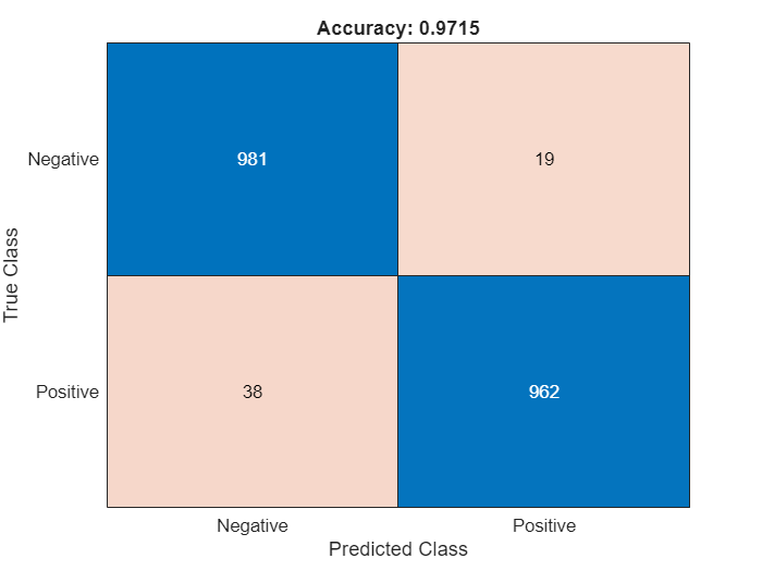
labelsTest = tdsTest.UnderlyingDatastores{1}.Labels ~= "Negative";Calculate the confusion matrix and the classification accuracy for the test set. The classification model in this example is accurate and predicts a small percentage of false positives and false negatives.
targetLabels = logical(labelsTest);
M = confusionmat(targetLabels,predictedLabels);
confusionchart(M,["Negative","Positive"])
acc = sum(diag(M)) / sum(M,"all");
title("Accuracy: "+acc);
Explain Classification Decisions
You can visualize the anomaly score map predicted by the PaDiM model as a heatmap overlaid on the image. You can use this localization of predicted anomalies to help explain why an image is classified as normal or anomalous. This approach is useful for identifying patterns in false negatives and false positives. You can use these patterns to identify strategies to improve the classifier performance.
Calculate Heatmap Display Range
Instead of scaling the heatmap for each image individually, visualize heatmap data using the same display range for all images in a data set. Doing so yields uniformly cool heatmaps for normal images and warm colors in anomalous regions for anomaly images.
Calculate a display range that reflects the range of anomaly score values observed in the calibration set. Apply the display range for all heatmaps in this example. Set the minimum value of the displayRange to 0. Set the maximum value of the display range by calculating the maximum score for each of the 200 calibration images, then selecting the 80th percentile of the maximums. Calculate the percentile value by using the prctile function.
maxScoresCal = mat2gray(maxScoresCal);
scoreMapRange = [0 prctile(maxScoresCal,80,"all")];
View Heatmap of Anomaly
Select an image of a correctly classified anomaly. This result is a true positive classification. Display the image.
idxTruePositive = find(targetLabels & predictedLabels);
dsTruePositive = subset(tdsTest,idxTruePositive);
dataTruePositive = preview(dsTruePositive);
imgTruePositive = dataTruePositive{1};
imshow(imgTruePositive)
title("True Positive Test Image")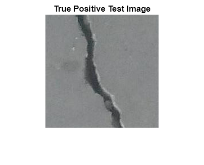
Obtain an anomaly score map of the true positive anomaly image. Normalize the anomaly scores to the minimum and maximum values of the calibration data set to match the range used to pick the threshold.
anomalyTestMapsRescaled = mat2gray(anomalyScoreMapsTest,[minScore maxScore]);
scoreMapTruePositive = anomalyTestMapsRescaled(:,:,1,idxTruePositive(1));
Display the heatmap as an overlay over the image by using the anomalyMapOverlayForConcreteAnomalyDetector helper function. This function is attached to the example as a supporting file.
imshow(anomalyMapOverlayForConcreteAnomalyDetector(imgTruePositive, ...
    scoreMapTruePositive,ScoreMapRange=scoreMapRange));
title("Heatmap Overlay of True Positive Result")

To quantitatively confirm the result, display the mean anomaly score of the true positive test image as predicted by the classifier. The value is greater than the anomaly score threshold.
disp("Mean anomaly score of test image: "+scoresTest(idxTruePositive(1)))Mean anomaly score of test image: 0.26587
View Heatmap of Normal Image
Select and display an image of a correctly classified normal image. This result is a true negative classification.
idxTrueNegative = find(~(targetLabels | predictedLabels));
dsTrueNegative = subset(tdsTest,idxTrueNegative);
dataTrueNegative = preview(dsTrueNegative);
imgTrueNegative = dataTrueNegative{1};
imshow(imgTrueNegative)
title("True Negative Test Image")
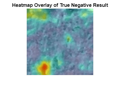
Obtain a heatmap of the normal image. Display the heatmap as an overlay over the image by using the anomalyMapOverlayForConcreteAnomalyDetector helper function. This function is attached to the example as a supporting file. Many true negative test images, such as this test image, have either small anomaly scores across the entire image or large anomaly scores in a localized portion of the image.
scoreMapTrueNegative = anomalyTestMapsRescaled(:,:,1,idxTrueNegative(1));
imshow(anomalyMapOverlayForConcreteAnomalyDetector(imgTrueNegative, ...
    scoreMapTrueNegative,ScoreMapRange=scoreMapRange))
title("Heatmap Overlay of True Negative Result")
To quantitatively confirm the result, display the mean anomaly score of the true positive test image as predicted by the classifier. The value is less than the anomaly score threshold.
disp("Mean anomaly score of test image: "+scoresTest(idxTrueNegative(1)))Mean anomaly score of test image: 0.22344
View Heatmaps of False Positive Images
False positives are images without crack anomalies that the network classifies as anomalous. Use the explanation from the PaDiM model to gain insight into the misclassifications.
Find false positive images from the test set. Display three false positive images as a montage.
idxFalsePositive = find(~targetLabels & predictedLabels);
dataFalsePositive = readall(subset(tdsTest,idxFalsePositive));
numelFalsePositive = length(idxFalsePositive);
numImages = min(numelFalsePositive,3);
if numelFalsePositive>0
    montage(dataFalsePositive(1:numImages,1),Size=[1,numImages],BorderSize=10);
    title("False Positives in Test Set")
end

Obtain heatmaps of the false positive images.
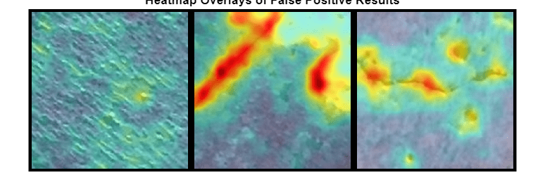
hmapOverlay = cell(1,numImages);
for idx = 1:numImages
    img = dataFalsePositive{idx,1};
    scoreMapFalsePositive = anomalyTestMapsRescaled(:,:,1,idxFalsePositive(idx));
    hmapOverlay{idx} = anomalyMapOverlayForConcreteAnomalyDetector(img, ...
        scoreMapFalsePositive,ScoreMapRange=scoreMapRange);
end
Display the heatmap overlays as a montage. The false positive images show features such as rocks that have similar visual characteristics to cracks. The anomaly scores are high in these localized regions. However, the training data set only labels images with cracks as anomalous, so the ground truth label for these images is Negative. Training a classifier that recognizes rocks and other non-crack defects as anomalous requires training data with non-crack defects labeled as anomalous.
if numelFalsePositive>0
    montage(hmapOverlay,Size=[1,numImages],BorderSize=10)
    title("Heatmap Overlays of False Positive Results")
end
Display the mean anomaly scores of the false positive test images as predicted by the PaDiM model. The mean scores are greater than the anomaly score threshold, resulting in misclassifications.
disp("Mean anomaly scores:"); scoresTest(idxFalsePositive(1:numImages))Mean anomaly scores:
ans = 3×1

    0.2432
    0.3120
    0.2625
View Heatmaps of False Negative Images
False negatives are images with crack anomalies that the network classifies as normal. Use the explanation from the PaDiM model to gain insights into the misclassifications.
Find any false negative images from the test set. Display three false negative images as a montage.
idxFalseNegative = find(targetLabels & ~predictedLabels);
dataFalseNegative = readall(subset(tdsTest,idxFalseNegative));
numelFalseNegative = length(idxFalseNegative);
numImages = min(numelFalseNegative,3);
if numelFalseNegative>0
    montage(dataFalseNegative(1:numImages,1),Size=[1,numImages],BorderSize=10);
    title("False Negatives in Test Set")
end

Obtain heatmaps of the false negative images.
hmapOverlay = cell(1,numImages);
for idx = 1:numImages
    img = dataFalseNegative{idx,1};
    scoreMapFalseNegative = anomalyTestMapsRescaled(:,:,1,idxFalseNegative(idx));
    hmapOverlay{idx} = anomalyMapOverlayForConcreteAnomalyDetector(img, ...
        scoreMapFalseNegative,ScoreMapRange=scoreMapRange);
end
Display the heatmap overlays as a montage. The PaDiM model predicts large anomaly scores around cracks, as expected.
if numelFalseNegative>0
    montage(hmapOverlay,Size=[1,numImages],BorderSize=10)
    title("Heatmap Overlays of False Negative Results")
end

Display the mean anomaly scores of the false negative test images as predicted by the PaDiM model. The mean scores are less than the anomaly score threshold, resulting in misclassifications.
disp("Mean anomaly scores:"); scoresTest(idxFalsePositive(1:numImages))Mean anomaly scores:
ans = 3×1

    0.2432
    0.3120
    0.2625
Supporting Functions
The concatenateEmbeddings helper function combines features extracted from three layers of ResNet-18 into one feature embedding vector. The features from the second and third blocks of ResNet-18 are resized to match the spatial resolution of the first block.
function XEmbeddings = concatenateEmbeddings(XFeatures1,XFeatures2,XFeatures3)
    XFeatures2Resize = imresize(XFeatures2,2,"nearest");
    XFeatures3Resize = imresize(XFeatures3,4,"nearest");
    XEmbeddings = cat(3,XFeatures1,XFeatures2Resize,XFeatures3Resize);
end
The calculateDistance helper function calculates the Mahalanobis distance between each embedding feature vector specified by XEmbeddings and the learned Gaussian distribution for the corresponding patch with mean specified by means and covariance matrix specified by covars.
function distances = calculateDistance(XEmbeddings,H,W,B,means,covars)
    distances = zeros([H*W 1 B]);
    for dIdx = 1:H*W
        distances(dIdx,1,:) = pdist2(squeeze(means(dIdx,:)), ...
            squeeze(XEmbeddings(dIdx,:,:)),"mahal",squeeze(covars(dIdx,:,:)));
    end
end
The createAnomalyScoreMap helper function creates an anomaly score map for each image with embeddings vectors specified by XEmbeddings. The createAnomalyScoreMap function reshapes and resizes the anomaly score map to match the size and resolution of the original input images.
function anomalyScoreMap = createAnomalyScoreMap(distances,H,W,B,targetImageSize)
    anomalyScoreMap = reshape(distances,[H W 1 B]);
    anomalyScoreMap = imresize(anomalyScoreMap,targetImageSize,"bilinear");
    for mIdx = 1:size(anomalyScoreMap,4)
        anomalyScoreMap(:,:,1,mIdx) = imgaussfilt(anomalyScoreMap(:,:,1,mIdx),4,FilterSize=33);
    end
end
References
[1] Defard, Thomas, Aleksandr Setkov, Angelique Loesch, and Romaric Audigier. “PaDiM: A Patch Distribution Modeling Framework for Anomaly Detection and Localization.” In Pattern Recognition. ICPR International Workshops and Challenges, 475–89. Lecture Notes in Computer Science. Cham, Switzerland: Springer International Publishing, 2021. https://doi.org/10.1007/978-3-030-68799-1_35.
[2] He, Kaiming, Xiangyu Zhang, Shaoqing Ren, and Jian Sun. “Deep Residual Learning for Image Recognition.” In 2016 IEEE Conference on Computer Vision and Pattern Recognition (CVPR), 770–78. Las Vegas, NV, USA: IEEE, 2016. https://doi.org/10.1109/CVPR.2016.90.
[3] ImageNet. https://www.image-net.org.
[4] Özgenel, Ç. F., and Arzu Gönenç Sorguç. “Performance Comparison of Pretrained Convolutional Neural Networks on Crack Detection in Buildings.” Taipei, Taiwan, 2018. https://doi.org/10.22260/ISARC2018/0094.
[5] Zhang, Lei, Fan Yang, Yimin Daniel Zhang, and Ying Julie Zhu. “Road Crack Detection Using Deep Convolutional Neural Network.” In 2016 IEEE International Conference on Image Processing (ICIP), 3708–12. Phoenix, AZ, USA: IEEE, 2016. https://doi.org/10.1109/ICIP.2016.7533052.
See Also
imageDatastore | predict (Deep Learning Toolbox) | perfcurve (Statistics and Machine Learning Toolbox) | confusionmat (Deep Learning Toolbox) | confusionchart (Deep Learning Toolbox)
Topics
- Detect Image Anomalies Using Explainable FCDD Network
- Classify Defects on Wafer Maps Using Deep Learning
- Datastores for Deep Learning (Deep Learning Toolbox)
- Preprocess Images for Deep Learning (Deep Learning Toolbox)