prctile

Percentiles of data set

Syntax

P = prctile(A,p)

P = prctile(A,p,"all")

P = prctile(A,p,dim)

P = prctile(A,p,vecdim)

P = prctile(___,"Method",method)

Description

P = prctile(A,p) returns percentiles of elements in input data A for the percentages p in the interval [0,100].

• If A is a vector, then P is a scalar or a vector with the same length as p. P(i) contains the p(i) percentile.

• If A is a matrix, then P is a row vector or a matrix, where the number of rows of P is equal to length(p). The ith row of P contains the p(i) percentiles of each column of A.

• If A is a multidimensional array, then P contains the percentiles computed along the first array dimension of size greater than 1.

P = prctile(A,p,"all") returns percentiles of all the elements in x.

P = prctile(A,p,dim) operates along the dimension dim. For example, if A is a matrix, then prctile(A,p,2) operates on the elements in each row.

P = prctile(A,p,vecdim) operates along the dimensions specified in the vector vecdim. For example, if A is a matrix, then prctile(A,p,[1 2]) operates on all the elements of A because every element of a matrix is contained in the array slice defined by dimensions 1 and 2.

P = prctile(___,"Method",method) returns either exact or approximate percentiles based on the value of method, using any of the input argument combinations in the previous syntaxes.

Examples

Percentiles of Data Vector

Calculate the percentile of a data set for a given percentage.

Generate a data set of size 7.

rng default % for reproducibility
A = randn(1,7)

A = 1×7

    0.5377    1.8339   -2.2588    0.8622    0.3188   -1.3077   -0.4336

Calculate the 42nd percentile of the elements of A.

P = prctile(A,42)

P = -0.1026

Percentiles of All Values

Find the percentiles of all the values in an array.

Create a 3-by-5-by-2 array.

rng default % for reproducibility
A = randn(3,5,2)

A = 
A(:,:,1) =

    0.5377    0.8622   -0.4336    2.7694    0.7254
    1.8339    0.3188    0.3426   -1.3499   -0.0631
   -2.2588   -1.3077    3.5784    3.0349    0.7147


A(:,:,2) =

   -0.2050    1.4090   -1.2075    0.4889   -0.3034
   -0.1241    1.4172    0.7172    1.0347    0.2939
    1.4897    0.6715    1.6302    0.7269   -0.7873

Find the 40th and 60th percentiles of all the elements of A.

P = prctile(A,[40 60],"all")

P = 2×1

    0.3307
    0.7213

P(1) is the 40th percentile of A, and P(2) is the 60th percentile of A.

Percentiles of Data Matrix

Calculate the percentiles along the columns and rows of a data matrix for specified percentages.

Generate a 5-by-5 data matrix.

A = (1:5)'*(2:6)

A = 5×5

     2     3     4     5     6
     4     6     8    10    12
     6     9    12    15    18
     8    12    16    20    24
    10    15    20    25    30

Calculate the 25th, 50th, and 75th percentiles for each column of A.

P = prctile(A,[25 50 75],1)

P = 3×5

    3.5000    5.2500    7.0000    8.7500   10.5000
    6.0000    9.0000   12.0000   15.0000   18.0000
    8.5000   12.7500   17.0000   21.2500   25.5000

Each column of matrix P contains the three percentiles for the corresponding column in matrix A. 7, 12, and 17 are the 25th, 50th, and 75th percentiles of the third column of A with elements 4, 8, 12, 16, and 20. P = prctile(A,[25 50 75]) returns the same result.

Calculate the 25th, 50th, and 75th percentiles along the rows of A.

P = prctile(A,[25 50 75],2)

P = 5×3

    2.7500    4.0000    5.2500
    5.5000    8.0000   10.5000
    8.2500   12.0000   15.7500
   11.0000   16.0000   21.0000
   13.7500   20.0000   26.2500

Each row of matrix P contains the three percentiles for the corresponding row in matrix A. 2.75, 4, and 5.25 are the 25th, 50th, and 75th percentiles of the first row of A with elements 2, 3, 4, 5, and 6.

Percentiles of Multidimensional Array

Find the percentiles of a multidimensional array along multiple dimensions.

Create a 3-by-5-by-2 array.

A = reshape(1:30,[3 5 2])

A = 
A(:,:,1) =

     1     4     7    10    13
     2     5     8    11    14
     3     6     9    12    15


A(:,:,2) =

    16    19    22    25    28
    17    20    23    26    29
    18    21    24    27    30

Calculate the 40th and 60th percentiles for each page of A by specifying dimensions 1 and 2 as the operating dimensions.

Ppage = prctile(A,[40 60],[1 2])

Ppage = 
Ppage(:,:,1) =

    6.5000
    9.5000


Ppage(:,:,2) =

   21.5000
   24.5000

Ppage(1,1,1) is the 40th percentile of the first page of A, and Ppage(2,1,1) is the 60th percentile of the first page of A.

Calculate the 40th and 60th percentiles of the elements in each A(:,i,:) slice by specifying dimensions 1 and 3 as the operating dimensions.

Pcol = prctile(A,[40 60],[1 3])

Pcol = 2×5

    2.9000    5.9000    8.9000   11.9000   14.9000
   16.1000   19.1000   22.1000   25.1000   28.1000

Pcol(1,4) is the 40th percentile of the elements in A(:,4,:), and Pcol(2,4) is the 60th percentile of the elements in A(:,4,:).

Percentiles of Tall Vector for Given Percentage

Calculate exact and approximate percentiles of a tall column vector for a given percentage.

When you perform calculations on tall arrays, MATLAB® uses either a parallel pool (default if you have Parallel Computing Toolbox™) or the local MATLAB session. To run the example using the local MATLAB session when you have Parallel Computing Toolbox, change the global execution environment by using the mapreducer function.

mapreducer(0)

Create a datastore for the airlinesmall data set. Treat "NA" values as missing data so that datastore replaces them with NaN values. Specify to work with the ArrTime variable.

ds = datastore("airlinesmall.csv","TreatAsMissing","NA", ...
    "SelectedVariableNames","ArrTime");

Create a tall table tt on top of the datastore, and extract the data from the tall table into a tall vector A.

tt = tall(ds)

tt =

  Mx1 tall table

    ArrTime
    _______

      735  
     1124  
     2218  
     1431  
      746  
     1547  
     1052  
     1134  
       :
       :

A = tt{:,:}

A =

  Mx1 tall double column vector

         735
        1124
        2218
        1431
         746
        1547
        1052
        1134
         :
         :

Calculate the exact 50th percentile of A. Because A is a tall column vector and p is a scalar, prctile returns the exact percentile value by default.

p = 50;
Pexact = prctile(A,p)

Pexact =

  tall double

    ?

Calculate the approximate 50th percentile of A. Specify the "approximate" method to use an approximation algorithm based on T-Digest for computing the percentile.

Papprox = prctile(A,p,"Method","approximate")

Papprox =

  MxNx... tall double array

    ?    ?    ?    ...
    ?    ?    ?    ...
    ?    ?    ?    ...
    :    :    :
    :    :    :

Evaluate the tall arrays and bring the results into memory by using gather.

[Pexact,Papprox] = gather(Pexact,Papprox)

Evaluating tall expression using the Local MATLAB Session:
- Pass 1 of 4: Completed in 1.2 sec
- Pass 2 of 4: Completed in 0.42 sec
- Pass 3 of 4: Completed in 0.7 sec
- Pass 4 of 4: Completed in 0.64 sec
Evaluation completed in 3.9 sec

Pexact = 1522

Papprox = 1.5220e+03

The values of the exact percentile and the approximate percentile are the same to the four digits shown.

Percentiles of Tall Matrix Along Different Dimensions

Calculate exact and approximate percentiles of a tall matrix for specified percentages along different dimensions.

When you perform calculations on tall arrays, MATLAB® uses either a parallel pool (default if you have Parallel Computing Toolbox™) or the local MATLAB session. To run the example using the local MATLAB session when you have Parallel Computing Toolbox, change the global execution environment by using the mapreducer function.

mapreducer(0)

Create a tall matrix A containing a subset of variables stored in varnames from the airlinesmall data set. See Percentiles of Tall Vector for Given Percentage for details about the steps to extract data from a tall array.

varnames = ["ArrDelay","ArrTime","DepTime","ActualElapsedTime"];
ds = datastore("airlinesmall.csv","TreatAsMissing","NA", ...
    "SelectedVariableNames",varnames);
tt = tall(ds);
A = tt{:,varnames}

A =

  Mx4 tall double matrix

           8         735         642          53
           8        1124        1021          63
          21        2218        2055          83
          13        1431        1332          59
           4         746         629          77
          59        1547        1446          61
           3        1052         928          84
          11        1134         859         155
          :          :            :           :
          :          :            :           :

When operating along a dimension that is not 1, the prctile function calculates exact percentiles only so that it can compute efficiently using a sorting-based algorithm (see Algorithms) instead of an approximation algorithm based on T-Digest.

Calculate the exact 25th, 50th, and 75th percentiles of A along the second dimension.

p = [25 50 75];
Pexact = prctile(A,p,2)

Pexact =

  MxNx... tall double array

    ?    ?    ?    ...
    ?    ?    ?    ...
    ?    ?    ?    ...
    :    :    :
    :    :    :

When the function operates along the first dimension and p is a vector of percentages, you must use the approximation algorithm based on t-digest to compute the percentiles. Using the sorting-based algorithm to find percentiles along the first dimension of a tall array is computationally intensive.

Calculate the approximate 25th, 50th, and 75th percentiles of A along the first dimension. Because the default dimension is 1, you do not need to specify a value for dim.

Papprox = prctile(A,p,"Method","approximate")

Papprox =

  MxNx... tall double array

    ?    ?    ?    ...
    ?    ?    ?    ...
    ?    ?    ?    ...
    :    :    :
    :    :    :

Evaluate the tall arrays and bring the results into memory by using gather.

[Pexact,Papprox] = gather(Pexact,Papprox);

Evaluating tall expression using the Local MATLAB Session:
- Pass 1 of 1: Completed in 2.9 sec
Evaluation completed in 3.7 sec

Show the first five rows of the exact 25th, 50th, and 75th percentiles along the second dimension of A.

Pexact(1:5,:)

ans = 5×3
103 ×

    0.0305    0.3475    0.6885
    0.0355    0.5420    1.0725
    0.0520    1.0690    2.1365
    0.0360    0.6955    1.3815
    0.0405    0.3530    0.6875

Each row of the matrix Pexact contains the three percentiles of the corresponding row in A. 30.5, 347.5, and 688.5 are the 25th, 50th, and 75th percentiles, respectively, of the first row in A.

Show the approximate 25th, 50th, and 75th percentiles of A along the first dimension.

Papprox

Papprox = 3×4
103 ×

   -0.0070    1.1150    0.9321    0.0700
         0    1.5220    1.3350    0.1020
    0.0110    1.9180    1.7400    0.1510

Each column of the matrix Papprox contains the three percentiles of the corresponding column in A. The first column of Papprox contains the percentiles for the first column of A.

Input Arguments

A — Input array

vector | matrix | multidimensional array

Input array, specified as a vector, matrix, or multidimensional array.

Data Types: double | single | duration

p — Percentages for which to compute percentiles

scalar | vector

Percentages for which to compute percentiles, specified as a scalar or vector of scalars from 0 to 100.

Example: 25

Example: [25, 50, 75]

Data Types: double | single

dim — Dimension to operate along

positive integer scalar

Dimension to operate along, specified as a positive integer scalar. If you do not specify the dimension, then the default is the first array dimension of size greater than 1.

Consider an input matrix A and a vector of percentages p:

• P = prctile(A,p,1) computes percentiles of the columns in A for the percentages in p.

• P = prctile(A,p,2) computes percentiles of the rows in A for the percentages in p.

Dimension dim indicates the dimension of P that has the same length as p.

Data Types: double | single | int8 | int16 | int32 | int64 | uint8 | uint16 | uint32 | uint64

vecdim — Vector of dimensions to operate along

vector of positive integers

Vector of dimensions to operate along, specified as a vector of positive integers. Each element represents a dimension of the input data.

The size of the output P in the smallest specified operating dimension is equal to the length of p. The size of P in the other operating dimensions specified in vecdim is 1. The size of P in all dimensions not specified in vecdim remains the same as the input data.

Consider a 2-by-3-by-3 input array A and the percentages p. prctile(A,p,[1 2]) returns a length(p)-by-1-by-3 array because 1 and 2 are the operating dimensions and min([1 2]) = 1. Each page of the returned array contains the percentiles of the elements on the corresponding page of A.

Data Types: double | single | int8 | int16 | int32 | int64 | uint8 | uint16 | uint32 | uint64

method — Method for calculating percentiles

"exact" (default) | "approximate"

Method for calculating percentiles, specified as one of these values:

• "exact" — Calculate exact percentiles with an algorithm that uses sorting.

• "approximate" — Calculate approximate percentiles with an algorithm that uses T-Digest for a double or single input array.

More About

Linear Interpolation

Linear interpolation uses linear polynomials to find y_i = f(x_i), the values of the underlying function Y = f(X) at the points in the vector or array x. Given the data points (x₁, y₁) and (x₂, y₂), where y₁ = f(x₁) and y₂ = f(x₂), linear interpolation finds y = f(x) for a given x between x₁ and x₂ as

$$y=f(x)=y_1+\frac{\left(x-x_1\right)}{\left(x_2-x_1\right)}\left(y_2-y_1\right).$$

Similarly, if the 100(1.5/n)th percentile is y_1.5/n and the 100(2.5/n)th percentile is y_2.5/n, then linear interpolation finds the 100(2.3/n)th percentile, y_2.3/n as

$$y_{\frac{2.3}{n}}=y_{\frac{1.5}{n}}+\frac{\left(\frac{2.3}{n}-\frac{1.5}{n}\right)}{\left(\frac{2.5}{n}-\frac{1.5}{n}\right)}\left(y_{\frac{2.5}{n}}-y_{\frac{1.5}{n}}\right).$$

T-Digest

T-digest [2] is a probabilistic data structure that is a sparse representation of the empirical cumulative distribution function (CDF) of a data set. T-digest is useful for computing approximations of rank-based statistics (such as percentiles and quantiles) from online or distributed data in a way that allows for controllable accuracy, particularly near the tails of the data distribution.

For data that is distributed in different partitions, t-digest computes quantile estimates (and percentile estimates) for each data partition separately, and then combines the estimates while maintaining a constant-memory bound and constant relative accuracy of computation ($$q(1-q)$$ for the qth quantile). For these reasons, t-digest is practical for working with tall arrays.

To estimate quantiles of an array that is distributed in different partitions, first build a t-digest in each partition of the data. A t-digest clusters the data in the partition and summarizes each cluster by a centroid value and an accumulated weight that represents the number of samples contributing to the cluster. T-digest uses large clusters (widely spaced centroids) to represent areas of the CDF that are near q = 0.5 and uses small clusters (tightly spaced centroids) to represent areas of the CDF that are near q = 0 and q = 1.

T-digest controls the cluster size by using a scaling function that maps a quantile q to an index k with a compression parameter δ. That is,

$$k(q,\delta )=\delta \cdot \left(\frac{{\sin }^{-1}(2q-1)}{\pi }+\frac{1}{2}\right),$$

where the mapping k is monotonic with minimum value k(0,δ) = 0 and maximum value k(1,δ) = δ. This figure shows the scaling function for δ = 10.

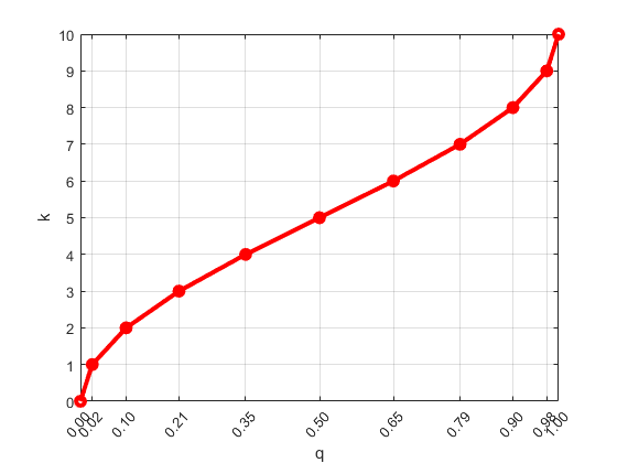
The scaling function translates the quantile q to the scaling factor k in order to give variable-size steps in q. As a result, cluster sizes are unequal (larger around the center quantiles and smaller near q = 0 and q = 1). The smaller clusters allow for better accuracy near the edges of the data.

To update a t-digest with a new observation that has a weight and location, find the cluster closest to the new observation. Then, add the weight and update the centroid of the cluster based on the weighted average, provided that the updated weight of the cluster does not exceed the size limitation.

You can combine independent t-digests from each partition of the data by taking a union of the t-digests and merging their centroids. To combine t-digests, first sort the clusters from all the independent t-digests in decreasing order of cluster weights. Then, merge neighboring clusters, when they meet the size limitation, to form a new t-digest.

Once you form a t-digest that represents the complete data set, you can estimate the endpoints (or boundaries) of each cluster in the t-digest and then use interpolation between the endpoints of each cluster to find accurate quantile estimates.

Algorithms

For an n-element vector A, prctile returns percentiles by using a sorting-based algorithm:

1. The sorted elements in A are taken as the 100(0.5/n)th, 100(1.5/n)th, ..., 100([n – 0.5]/n)th percentiles. For example:

   • For a data vector of five elements such as {6, 3, 2, 10, 1}, the sorted elements {1, 2, 3, 6, 10} respectively correspond to the 10th, 30th, 50th, 70th, and 90th percentiles.

   • For a data vector of six elements such as {6, 3, 2, 10, 8, 1}, the sorted elements {1, 2, 3, 6, 8, 10} respectively correspond to the (50/6)th, (150/6)th, (250/6)th, (350/6)th, (450/6)th, and (550/6)th percentiles.

2. prctile uses linear interpolation to compute percentiles for percentages between 100(0.5/n) and 100([n – 0.5]/n).

3. prctile assigns the minimum or maximum values of the elements in A to the percentiles corresponding to the percentages outside that range.

prctile treats NaNs as missing values and removes them.

References

[1] Langford, E. “Quartiles in Elementary Statistics”, Journal of Statistics Education. Vol. 14, No. 3, 2006.

[2] Dunning, T., and O. Ertl. “Computing Extremely Accurate Quantiles Using T-Digests.” August 2017.

Extended Capabilities

Tall Arrays

Calculate with arrays that have more rows than fit in memory.

Usage notes and limitations:

• P = prctile(A,p) returns the exact percentiles (using a sorting-based algorithm) only if A is a tall numeric column vector.

• P = prctile(A,p,dim) returns the exact percentiles only when one of these conditions exists:

  • A is a tall numeric column vector.

  • A is a tall numeric array and dim is not 1. For example, prctile(A,p,2) returns the exact percentiles along the rows of the tall array A.

  If A is a tall numeric array and dim is 1, then you must specify method as "approximate" to use an approximation algorithm based on T-Digest for computing the percentiles. For example, prctile(A,p,1,"Method","approximate") returns the approximate percentiles along the columns of the tall array A.

• P = prctile(A,p,vecdim) returns the exact percentiles only when one of these conditions exists:

  • A is a tall numeric column vector.

  • A is a tall numeric array and vecdim does not include 1. For example, if A is a 3-by-5-by-2 array, then prctile(A,p,[2,3]) returns the exact percentiles of the elements in each A(i,:,:) slice.

  • A is a tall numeric array and vecdim includes 1 and all the dimensions of A with a size greater than 1. For example, if A is a 10-by-1-by-4 array, then prctile(A,p,[1 3]) returns the exact percentiles of the elements in A(:,1,:).

  If A is a tall numeric array and vecdim includes 1 but does not include all the dimensions of A with a size greater than 1, then you must specify method as "approximate" to use the approximation algorithm. For example, if A is a 10-by-1-by-4 array, you can use prctile(A,p,[1 2],"Method","approximate") to find the approximate percentiles of each page of A.

For more information, see Tall Arrays.

C/C++ Code Generation

Generate C and C++ code using MATLAB® Coder™.

Usage notes and limitations:

• The "all" and vecdim inputs are not supported.

• The Method name-value argument is not supported.

• The dim input argument must be a compile-time constant.

• If you do not specify the dim input argument, the working (or operating) dimension can be different in the generated code. As a result, run-time errors can occur. For more details, see Automatic dimension restriction (MATLAB Coder).

• If the output P is a vector, the orientation of P differs from MATLAB^® when all of these conditions are true:

  • You do not supply dim.

  • A is a variable-size array, and not a variable-size vector, at compile time, but A is a vector at run time.

  • The orientation of the vector A does not match the orientation of the vector p.

  In this case, the output P matches the orientation of A, not the orientation of p.

GPU Arrays

Accelerate code by running on a graphics processing unit (GPU) using Parallel Computing Toolbox™.

Usage notes and limitations:

• The "all" and vecdim inputs are not supported.

• The Method name-value argument is not supported.

For more information, see Run MATLAB Functions on a GPU (Parallel Computing Toolbox).

Distributed Arrays

Partition large arrays across the combined memory of your cluster using Parallel Computing Toolbox™.

Usage notes and limitations:

• Duration inputs are not supported.

For more information, see Run MATLAB Functions with Distributed Arrays (Parallel Computing Toolbox).

Version History

Introduced before R2006a

R2022b: Improved performance with small input data

The prctile function shows improved performance due to faster input parsing. The performance improvement is most significant when input parsing is a greater portion of the computation time. This situation occurs when:

• The size of the input data is small.

• The number of percentages for which to compute percentiles is small.

• Computation is along the default operating dimension.

For example, this code calculates four percentiles for a 3000-element matrix. The code is about 5x faster than in the previous release.

function timingPrctile
A = rand(300,10);
for k = 1:3e3
  P = prctile(A,[20 40 60 80]);
end
end

The approximate execution times are:

R2022a: 1.0 s

R2022b: 0.2 s

The code was timed on a Windows^® 10, Intel^® Xeon^® CPU E5-1650 v4 @ 3.60 GHz test system using the timeit function:

timeit(@timingPrctile)

R2022a: Moved to MATLAB from Statistics and Machine Learning Toolbox

Previously, prctile required Statistics and Machine Learning Toolbox™.