Portfolio
Create Portfolio object for mean-variance portfolio optimization and analysis
Description
Use the Portfolio function to create a
Portfolio object for mean-variance portfolio
optimization.
The main workflow for portfolio optimization is to create an instance of a
Portfolio object that completely specifies a portfolio
optimization problem and to operate on the Portfolio object using
supported functions to obtain and analyze efficient portfolios. For details on this
workflow, see Portfolio Object Workflow.
You can use the Portfolio object in several ways. To set up a
portfolio optimization problem in a Portfolio object, the simplest
syntax is:
p = Portfolio;
Portfolio object, p, such that
all object properties are empty. The Portfolio object also accepts collections of name-value pair
arguments for properties and their values. The Portfolio object
accepts inputs for properties with the general
syntax:
p = Portfolio('property1',value1,'property2',value2, ... );If a Portfolio object exists, the syntax permits the first (and
only the first argument) of the Portfolio object to be an existing
object with subsequent name-value pair arguments for properties to be added or modified.
For example, given an existing Portfolio object in
p, the general syntax
is:
p = Portfolio(p,'property1',value1,'property2',value2, ... );
Input argument names are not case-sensitive, but must be completely specified. In
addition, several properties can be specified with alternative argument names (see Shortcuts for Property Names).
The Portfolio object tries to detect problem dimensions from the
inputs and, once set, subsequent inputs can undergo various scalar or matrix expansion
operations that simplify the overall process to formulate a problem. In addition, a
Portfolio object is a value object so that, given portfolio
p, the following code creates two objects, p
and q, that are
distinct:
q = Portfolio(p, ...)
After creating a Portfolio object, you can use the associated
object functions to set portfolio constraints, analyze the efficient frontier, and
validate the portfolio model.
For more detailed information on the theoretical basis for mean-variance optimization, see Portfolio Optimization Theory.
Creation
Description
p = PortfolioPortfolio object for mean-variance portfolio
optimization and analysis. You can then add elements to the
Portfolio object using the supported "add" and "set"
functions. For more information, see Creating the Portfolio Object.
p = Portfolio(Name,Value)Portfolio object (p) and
sets Properties using name-value
pairs. For example, p =
Portfolio('AssetList',Assets(1:12)). You can specify multiple
name-value pairs.
p = Portfolio(p,Name,Value)Portfolio object (p) using a
previously created Portfolio object
p and sets Properties using name-value
pairs. You can specify multiple name-value pairs.
Input Arguments
Output Arguments
Properties
Object Functions
setAssetList | Set up list of identifiers for assets |
setInitPort | Set up initial or current portfolio |
setDefaultConstraints | Set up portfolio constraints with nonnegative weights that sum to 1 |
getAssetMoments | Obtain mean and covariance of asset returns from Portfolio object |
setAssetMoments | Set moments (mean and covariance) of asset returns for Portfolio object |
estimateAssetMoments | Estimate mean and covariance of asset returns from data |
setCosts | Set up proportional transaction costs for portfolio |
addEquality | Add linear equality constraints for portfolio weights to existing constraints |
addGroupRatio | Add group ratio constraints for portfolio weights to existing group ratio constraints |
addGroups | Add group constraints for portfolio weights to existing group constraints |
addInequality | Add linear inequality constraints for portfolio weights to existing constraints |
getBounds | Obtain bounds for portfolio weights from portfolio object |
getBudget | Obtain budget constraint bounds from portfolio object |
getCosts | Obtain buy and sell transaction costs from portfolio object |
getEquality | Obtain equality constraint arrays from portfolio object |
getGroupRatio | Obtain group ratio constraint arrays from portfolio object |
getGroups | Obtain group constraint arrays from portfolio object |
getInequality | Obtain inequality constraint arrays from portfolio object |
getOneWayTurnover | Obtain one-way turnover constraints from portfolio object |
setGroups | Set up group constraints for portfolio weights |
setInequality | Set up linear inequality constraints for portfolio weights |
setBounds | Set up bounds for portfolio weights for portfolio |
setBudget | Set up budget constraints for portfolio |
setConditionalBudget | Set up conditional budget constraints for portfolio |
setCosts | Set up proportional transaction costs for portfolio |
setEquality | Set up linear equality constraints for portfolio weights |
setGroupRatio | Set up group ratio constraints for portfolio weights |
setOneWayTurnover | Set up one-way portfolio turnover constraints |
setTurnover | Set up maximum portfolio turnover constraint |
setTrackingPort | Set up benchmark portfolio for tracking error constraint |
setTrackingError | Set up maximum portfolio tracking error constraint |
setMinMaxNumAssets | Set cardinality constraints on the number of assets invested in a portfolio |
checkFeasibility | Check feasibility of input portfolios against portfolio object |
estimateBounds | Estimate global lower and upper bounds for set of portfolios |
estimateFrontier | Estimate specified number of optimal portfolios on the efficient frontier |
estimateFrontierByReturn | Estimate optimal portfolios with targeted portfolio returns |
estimateFrontierByRisk | Estimate optimal portfolios with targeted portfolio risks |
estimateFrontierLimits | Estimate optimal portfolios at endpoints of efficient frontier |
plotFrontier | Plot efficient frontier |
estimateMaxSharpeRatio | Estimate efficient portfolio to maximize Sharpe ratio for Portfolio object |
estimatePortMoments | Estimate moments of portfolio returns for Portfolio object |
estimatePortReturn | Estimate mean of portfolio returns |
estimatePortRisk | Estimate portfolio risk according to risk proxy associated with corresponding object |
estimateCustomObjectivePortfolio | Estimate optimal portfolio for user-defined objective function for
Portfolio object |
setSolver | Choose main solver and specify associated solver options for portfolio optimization |
setSolverMINLP | Choose mixed integer nonlinear programming (MINLP) solver for portfolio optimization |
Examples
You can create a Portfolio object, p, with no input arguments and display it using disp.
p = Portfolio;
disp(p);
  Portfolio with properties:

                       BuyCost: []
                      SellCost: []
                  RiskFreeRate: []
                     AssetMean: []
                    AssetCovar: []
                 TrackingError: []
                  TrackingPort: []
                      Turnover: []
                   BuyTurnover: []
                  SellTurnover: []
                          Name: []
                     NumAssets: []
                     AssetList: []
                      InitPort: []
                   AInequality: []
                   bInequality: []
                     AEquality: []
                     bEquality: []
                    LowerBound: []
                    UpperBound: []
                   LowerBudget: []
                   UpperBudget: []
                   GroupMatrix: []
                    LowerGroup: []
                    UpperGroup: []
                        GroupA: []
                        GroupB: []
                    LowerRatio: []
                    UpperRatio: []
                  MinNumAssets: []
                  MaxNumAssets: []
    ConditionalBudgetThreshold: []
        ConditionalUpperBudget: []
                     BoundType: []
This approach provides a way to set up a portfolio optimization problem with the Portfolio function. You can then use the associated set functions to set and modify collections of properties in the Portfolio object.
You can use the Portfolio object directly to set up a “standard” portfolio optimization problem, given a mean and covariance of asset returns in the variables m and C.
m = [ 0.05; 0.1; 0.12; 0.18 ];
C = [ 0.0064 0.00408 0.00192 0;
    0.00408 0.0289 0.0204 0.0119;
    0.00192 0.0204 0.0576 0.0336;
    0 0.0119 0.0336 0.1225 ];

p = Portfolio('assetmean', m, 'assetcovar', C, ...
'lowerbudget', 1, 'upperbudget', 1, 'lowerbound', 0)
p =
Portfolio with properties:
BuyCost: []
SellCost: []
RiskFreeRate: []
AssetMean: [4×1 double]
AssetCovar: [4×4 double]
TrackingError: []
TrackingPort: []
Turnover: []
BuyTurnover: []
SellTurnover: []
Name: []
NumAssets: 4
AssetList: []
InitPort: []
AInequality: []
bInequality: []
AEquality: []
bEquality: []
LowerBound: [4×1 double]
UpperBound: []
LowerBudget: 1
UpperBudget: 1
GroupMatrix: []
LowerGroup: []
UpperGroup: []
GroupA: []
GroupB: []
LowerRatio: []
UpperRatio: []
MinNumAssets: []
MaxNumAssets: []
ConditionalBudgetThreshold: []
ConditionalUpperBudget: []
BoundType: []
Note that the LowerBound property value undergoes scalar expansion since AssetMean and AssetCovar provide the dimensions of the problem.
Using a sequence of steps is an alternative way to accomplish the same task of setting up a “standard” portfolio optimization problem, given a mean and covariance of asset returns in the variables m and C (which also illustrates that argument names are not case sensitive).
m = [ 0.05; 0.1; 0.12; 0.18 ];
C = [ 0.0064 0.00408 0.00192 0;
    0.00408 0.0289 0.0204 0.0119;
    0.00192 0.0204 0.0576 0.0336;
    0 0.0119 0.0336 0.1225 ];

p = Portfolio;
p = Portfolio(p, 'assetmean', m, 'assetcovar', C);
p = Portfolio(p, 'lowerbudget', 1, 'upperbudget', 1);
p = Portfolio(p, 'lowerbound', 0);

plotFrontier(p);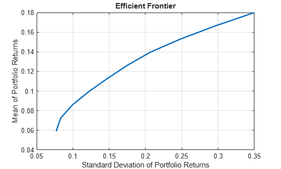
This way works because the calls to Portfolio are in this particular order. In this case, the call to initialize AssetMean and AssetCovar provides the dimensions for the problem. If you were to do this step last, you would have to explicitly dimension the LowerBound property as follows:
m = [ 0.05; 0.1; 0.12; 0.18 ];
C = [ 0.0064 0.00408 0.00192 0;
    0.00408 0.0289 0.0204 0.0119;
    0.00192 0.0204 0.0576 0.0336;
    0 0.0119 0.0336 0.1225 ];

p = Portfolio;
p = Portfolio(p, 'LowerBound', zeros(size(m)));
p = Portfolio(p, 'LowerBudget', 1, 'UpperBudget', 1);
p = Portfolio(p, 'AssetMean', m, 'AssetCovar', C);

plotFrontier(p);
If you did not specify the size of LowerBound but, instead, input a scalar argument, the Portfolio object assumes that you are defining a single-asset problem and produces an error at the call to set asset moments with four assets.
You can create a Portfolio object, p with Portfolio using shortcuts for property names.
m = [ 0.05; 0.1; 0.12; 0.18 ];
C = [ 0.0064 0.00408 0.00192 0;
    0.00408 0.0289 0.0204 0.0119;
    0.00192 0.0204 0.0576 0.0336;
    0 0.0119 0.0336 0.1225 ];

p = Portfolio('mean', m, 'covar', C, 'budget', 1, 'lb', 0)
p =
Portfolio with properties:
BuyCost: []
SellCost: []
RiskFreeRate: []
AssetMean: [4×1 double]
AssetCovar: [4×4 double]
TrackingError: []
TrackingPort: []
Turnover: []
BuyTurnover: []
SellTurnover: []
Name: []
NumAssets: 4
AssetList: []
InitPort: []
AInequality: []
bInequality: []
AEquality: []
bEquality: []
LowerBound: [4×1 double]
UpperBound: []
LowerBudget: 1
UpperBudget: 1
GroupMatrix: []
LowerGroup: []
UpperGroup: []
GroupA: []
GroupB: []
LowerRatio: []
UpperRatio: []
MinNumAssets: []
MaxNumAssets: []
ConditionalBudgetThreshold: []
ConditionalUpperBudget: []
BoundType: []
Although not recommended, you can set properties directly, however no error-checking is done on your inputs.
m = [ 0.05; 0.1; 0.12; 0.18 ];
C = [ 0.0064 0.00408 0.00192 0;
    0.00408 0.0289 0.0204 0.0119;
    0.00192 0.0204 0.0576 0.0336;
    0 0.0119 0.0336 0.1225 ];

p = Portfolio;
p.NumAssets = numel(m);
p.AssetMean = m;
p.AssetCovar = C;
p.LowerBudget = 1;
p.UpperBudget = 1;
p.LowerBound = zeros(size(m));
disp(p)
Portfolio with properties:
BuyCost: []
SellCost: []
RiskFreeRate: []
AssetMean: [4×1 double]
AssetCovar: [4×4 double]
TrackingError: []
TrackingPort: []
Turnover: []
BuyTurnover: []
SellTurnover: []
Name: []
NumAssets: 4
AssetList: []
InitPort: []
AInequality: []
bInequality: []
AEquality: []
bEquality: []
LowerBound: [4×1 double]
UpperBound: []
LowerBudget: 1
UpperBudget: 1
GroupMatrix: []
LowerGroup: []
UpperGroup: []
GroupA: []
GroupB: []
LowerRatio: []
UpperRatio: []
MinNumAssets: []
MaxNumAssets: []
ConditionalBudgetThreshold: []
ConditionalUpperBudget: []
BoundType: []
Create efficient portfolios:
load CAPMuniverse

p = Portfolio('AssetList',Assets(1:12));
p = estimateAssetMoments(p, Data(:,1:12),'missingdata',true);
p = setDefaultConstraints(p);
plotFrontier(p);
pwgt = estimateFrontier(p, 5);

pnames = cell(1,5);
for i = 1:5
	pnames{i} = sprintf('Port%d',i);
end

Blotter = dataset([{pwgt},pnames],'obsnames',p.AssetList);

disp(Blotter);
            Port1         Port2         Port3         Port4         Port5
    AAPL      0.017926      0.058247      0.097816       0.12955    0
    AMZN     1.782e-13    1.5832e-11    2.1265e-10    2.0669e-11    0
    CSCO    1.3365e-14    7.4305e-13    5.1756e-11     2.798e-12    0
    DELL     0.0041906    4.0213e-10    2.9535e-09    1.0249e-10    0
    EBAY    1.2686e-14    1.6093e-12    1.0334e-10    1.0811e-11    0
    GOOG       0.16144       0.35678       0.55228       0.75116    1
    HPQ       0.052566      0.032302      0.011186    6.1882e-09    0
    IBM        0.46422       0.36045       0.25577       0.11928    0
    INTC    4.5883e-14    2.0534e-11     3.845e-08    1.8432e-08    0
    MSFT       0.29966       0.19222      0.082949    1.7512e-09    0
    ORCL    1.9196e-14    1.5317e-12    1.0064e-10    7.6664e-12    0
    YHOO    5.4342e-15    1.1905e-13    1.3146e-11    3.7126e-13    0
This example shows how to solve a mean-variance portfolio optimization problem with constraints in the number of selected assets or conditional (semicontinuous) bounds. To solve this problem, you can use a Portfolio object along with different mixed integer nonlinear programming (MINLP) solvers.
Mean-Variance Portfolio
Load the returns data in CAPMuniverse.mat. Then, create a mean-variance Portfolio object with default constraints and a long-only portfolio whose weights sum to 1. For this example, you can define the feasible region of weights as
% Load data
load CAPMuniverse.mat

% Create a mean-variance Portfolio object with default constraints.
p = Portfolio(AssetList=Assets(1:12));
p = estimateAssetMoments(p,Data(:,1:12));
p = setDefaultConstraints(p);
Include binary variables for this scenario by setting conditional (semicontinuous) bounds. Conditional bounds are those such that or . In this example, for all assets.
% Set conditional bounds
condLB = 0.1;
condUB = 0.5;
p = setBounds(p,condLB,condUB,BoundType="conditional");
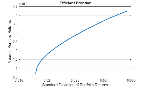
Use estimateFrontier to estimate a set of portfolios on the efficient frontier. The efficient frontier is a curve that shows the trade-off between the return and risk achieved by Pareto-optimal portfolios. For a given return level, the portfolio on the efficient frontier is the one that minimizes the risk while maintaining the desired return. Conversely, for a given risk level, the portfolio on the efficient frontier is the one that maximizes return while maintaining the desired risk level.
% Compute the efficient frontier.
pwgt = estimateFrontier(p)
pwgt = 12×10
0 0 0.1000 0.1253 0.1745 0.2236 0.2715 0.3327 0.4111 0.5000
0 0 0 0 0 0 0 0 0 0
0 0 0 0 0 0 0 0 0 0
0.1350 0 0 0 0 0 0 0 0 0
0 0 0 0 0 0 0 0 0 0
0.1000 0.1450 0.1406 0.1910 0.2344 0.2778 0.3200 0.3726 0.4415 0.5000
0.1000 0.1609 0.1642 0.2121 0.2415 0.2709 0.3085 0.2947 0.1474 0
0.2354 0.1875 0.1290 0 0 0 0 0 0 0
0 0 0 0 0 0 0 0 0 0
0.4296 0.4066 0.3662 0.3717 0.2496 0.1277 0 0 0 0
0 0.1000 0.1000 0.1000 0.1000 0.1000 0.1000 0 0 0
0 0 0 0 0 0 0 0 0 0
% Compute risk and returns of the portfolios on the efficient frontier.
[rsk,ret] = estimatePortMoments(p,pwgt)
rsk = 10×1
0.0076
0.0080
0.0085
0.0094
0.0105
0.0117
0.0132
0.0147
0.0168
0.0193
ret = 10×1

    0.0008
    0.0012
    0.0017
    0.0021
    0.0026
    0.0030
    0.0034
    0.0039
    0.0043
    0.0048
Plot the weights from the frontier estimation using plotFrontier. The resulting curve is piece-wise concave with vertical jumps (discontinuities) between the concave intervals.
% Plot the efficient frontier.
plotFrontier(p,pwgt)
Changing MINLP Solvers
In the previous section, you use the default solver for estimateFrontier. However, you can solve mixed-integer portfolio problems using any of the three algorithms supported by setSolverMINLP: OuterApproximation, ExtendedCP, and TrustRegionCP. Furthermore, the OuterApproximation algorithm accepts an additional name-value argument (ExtendedFormulation) for Portfolio problems, which reformulates problems with quadratic functions to work in an extended space that usually decreases the computation time. All algorithms, including the extended formulation variation of the OuterApproximation algorithm, return the same values within numerical accuracy. The available solvers are:
OuterApproximation— The default algorithm, which is robust and usually faster thanExtenedCPOuterApproximationwithExtendedFormulationset totrue— A robust algorithm that is usually faster than other algorithms, but only supported forPortfolioobject problemsExtendedCP— The most robust solver, but usually the slowestTrustRegionCP— The fastest algorithm, but one that is less robust and may provide suboptimal solutions
For more information on solvers for mixed-integer portfolio problems, see Choose MINLP Solvers for Portfolio Problems.
To change the MINLP solvers, use setSolverMINLP.
% Select the extended formulation version of 'OuterApproximation' as the
% solver.
p_EOA = setSolverMINLP(p,'OuterApproximation',...
    ExtendedFormulation=true);
pwgt_EOA = estimateFrontier(p_EOA);
[rskEOA,retEOA] = estimatePortMoments(p_EOA,pwgt_EOA);

% Select 'TrustRegionCP' as the solver.
p_TR = setSolverMINLP(p,'TrustRegionCP');
pwgt_TR = estimateFrontier(p_TR);
[rskTR,retTR] = estimatePortMoments(p_TR,pwgt_TR);

% Select 'ExtendedCP' as the solver using 'midway' cuts as 'CutGeneration'.
p_ECP = setSolverMINLP(p,'ExtendedCP','CutGeneration','midway');
pwgt_ECP = estimateFrontier(p_ECP);
[rskECP,retECP] = estimatePortMoments(p_ECP,pwgt_ECP);
Compare the returns and risks obtained by the portfolios on the efficient frontier from the different solvers. These are same within a numerical accuracy, where the absolute difference is .
retTable = table(ret,retEOA,retTR,retECP,...
    'VariableNames',{'OA','EOA','TR','ECP'})
retTable=10×4 table
        OA           EOA            TR           ECP
    __________    __________    __________    __________

    0.00078336    0.00078336    0.00078336    0.00078344
     0.0012267     0.0012267     0.0012267     0.0012267
       0.00167       0.00167       0.00167       0.00167
     0.0021133     0.0021133     0.0021133     0.0021133
     0.0025566     0.0025566     0.0025566     0.0025566
     0.0029999     0.0029999     0.0029999     0.0029999
     0.0034432     0.0034432     0.0034432     0.0034432
     0.0038865     0.0038865     0.0038865     0.0038865
     0.0043298     0.0043298     0.0043298     0.0043298
     0.0047731     0.0047731     0.0047731     0.0047731
rskTable = table(rsk,rskEOA,rskTR,rskECP,...
    'VariableNames',{'OA','EOA','TR','ECP'})
rskTable=10×4 table
       OA           EOA          TR           ECP
    _________    _________    _________    _________

    0.0075778    0.0075778    0.0075778    0.0075778
    0.0080234    0.0080234    0.0080235    0.0080235
    0.0085488    0.0085488    0.0086052    0.0085489
    0.0094024    0.0094024    0.0094051    0.0094025
     0.010456     0.010456     0.010456     0.010456
     0.011727     0.011727     0.011776     0.011728
     0.013155     0.013155     0.013155     0.013155
     0.014729     0.014729     0.014729     0.014729
     0.016764     0.016764     0.016764     0.016764
     0.019273     0.019273     0.019273     0.019273
% Compare the risks from the different OuterApproximation formulations.
norm(rskTable.OA-rskTable.EOA,Inf) <= 1e-4
ans = logical
1
More About
References
[1] For a complete list of references for the Portfolio object, see Portfolio Optimization.
Version History
Introduced in R2011aSee Also
plotFrontier | estimateFrontier | PortfolioCVaR | PortfolioMAD | nearcorr | covarianceShrinkage | covarianceDenoising
Topics
- Creating the Portfolio Object
- Working with Portfolio Constraints Using Defaults
- Estimate Efficient Portfolios for Entire Efficient Frontier for Portfolio Object
- Estimate Efficient Frontiers for Portfolio Object
- Asset Allocation Case Study
- Portfolio Optimization Examples Using Financial Toolbox
- Portfolio Optimization with Semicontinuous and Cardinality Constraints
- Black-Litterman Portfolio Optimization Using Financial Toolbox
- Portfolio Optimization Using Factor Models
- Bond Portfolio Optimization Using Portfolio Object
- Use Extended Formulation of OuterApproximation Solver Type
- Single Period Goal-Based Wealth Management
- Dynamic Portfolio Allocation in Goal-Based Wealth Management for Multiple Time Periods
- Multiperiod Goal-Based Wealth Management Using Reinforcement Learning
- Adding Constraints to Satisfy UCITS Directive
- Portfolio Optimization Theory
- Portfolio Object Workflow
- Portfolio Object Properties and Functions
- Working with Portfolio Objects
- Setting and Getting Properties
- Displaying Portfolio Objects
- Saving and Loading Portfolio Objects
- Estimating Efficient Portfolios and Frontiers
- Arrays of Portfolio Objects
- Subclassing Portfolio Objects
- Conventions for Representation of Data
- Supported Constraints for Portfolio Optimization Using Portfolio Objects
- Role of Convexity in Portfolio Problems
- When to Use Portfolio Objects Over Optimization Toolbox
- Solver Guidelines for Portfolio Objects
- Choosing and Controlling the Solver for Mean-Variance Portfolio Optimization
- Choose MINLP Solvers for Portfolio Problems
External Websites
- Getting Started with Portfolio Optimization (4 min 12 sec)
- Portfolio Optimization Across Risk, Returns, and Climate (58 min 22 sec)
- MATLAB for Advanced Portfolio Construction and Stock Selection Models (30 min 28 sec)
- Advanced Software Development Techniques for Finance (46 min 04 sec)
- Managing and Fine-Tuning Portfolio Optimization Workflows with Experiment Manager (20 min 21 sec)