estimateMaxSharpeRatio
Estimate efficient portfolio to maximize Sharpe ratio for Portfolio object
Syntax
Description
Examples
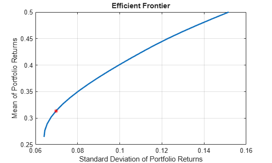
Estimate the efficient portfolio that maximizes the Sharpe ratio. The estimateMaxSharpeRatio function maximizes the Sharpe ratio among portfolios on the efficient frontier. This example uses the default 'direct' method to estimate the maximum Sharpe ratio. For more information on the 'direct' method, see Algorithms.
p = Portfolio('AssetMean',[0.3, 0.1, 0.5], 'AssetCovar',...
[0.01, -0.010,  0.004; -0.010,  0.040, -0.002;  0.004, -0.002,  0.023]);
p = setDefaultConstraints(p);
plotFrontier(p, 20);
weights = estimateMaxSharpeRatio(p);
[risk, ret] = estimatePortMoments(p, weights);
hold on
plot(risk,ret,'*r');
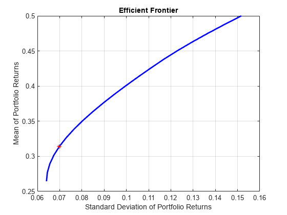
Estimate the efficient portfolio that maximizes the Sharpe ratio. The estimateMaxSharpeRatio function maximizes the Sharpe ratio among portfolios on the efficient frontier. This example uses the 'direct' method for a Portfolio object (p) that does not specify a tracking error and only uses linear constraints. The setSolver function is used to control the SolverType and SolverOptions. In this case, the SolverType is quadprog. For more information on the 'direct' method, see Algorithms.
p = Portfolio('AssetMean',[0.3, 0.1, 0.5], 'AssetCovar',...
[0.01, -0.010,  0.004; -0.010,  0.040, -0.002;  0.004, -0.002,  0.023]);
p = setDefaultConstraints(p);
plotFrontier(p, 20);
p = setSolver(p,'quadprog','Display','off','ConstraintTolerance',1.0e-8,'OptimalityTolerance',1.0e-8,'StepTolerance',1.0e-8,'MaxIterations',10000);
weights = estimateMaxSharpeRatio(p);
[risk, ret] = estimatePortMoments(p, weights);
hold on
plot(risk,ret,'*r');
Estimate the efficient portfolio that maximizes the Sharpe ratio. The estimateMaxSharpeRatio function maximizes the Sharpe ratio among portfolios on the efficient frontier. This example uses the 'direct' method for a Portfolio object (p) that specifies a tracking error uses nonlinear constraints. The setSolver function is used to control the SolverType and SolverOptions. In this case fmincon is the SolverType.
p = Portfolio('AssetMean',[0.3, 0.1, 0.5], 'AssetCovar',...
[0.01, -0.010,  0.004; -0.010,  0.040, -0.002;  0.004, -0.002,  0.023],'lb', 0,'budget', 1);
plotFrontier(p, 20);

p = setSolver(p, 'fmincon', 'Display', 'off', 'Algorithm', 'sqp', ...
        'SpecifyObjectiveGradient', true, 'SpecifyConstraintGradient', true, ...
        'ConstraintTolerance', 1.0e-8, 'OptimalityTolerance', 1.0e-8, 'StepTolerance', 1.0e-8);

weights = estimateMaxSharpeRatio(p);

te = 0.08;
p = setTrackingError(p,te,weights);

[risk, ret] = estimatePortMoments(p,weights);
hold on
plot(risk,ret,'*r');
![]()
The estimateMaxSharpeRatio function maximizes the Sharpe ratio among portfolios on the efficient frontier. In the case of Portfolio with a risk-free asset, there are multiple efficient portfolios that maximize the Sharpe ratio on the capital asset line. Because of the nature of 'direct' and 'iterative' methods, the portfolio weights (pwgts) output from each of these methods might be different, but the Sharpe ratio is the same. This example demonstrates the scenario where the pwgts are different and the Sharpe ratio is the same.
load BlueChipStockMoments

mret = MarketMean;
mrsk = sqrt(MarketVar);
cret = CashMean;
crsk = sqrt(CashVar);

p = Portfolio('AssetList', AssetList, 'RiskFreeRate', CashMean);
p = setAssetMoments(p, AssetMean, AssetCovar);

p = setInitPort(p, 1/p.NumAssets);
[ersk, eret] = estimatePortMoments(p, p.InitPort);

p = setDefaultConstraints(p);
pwgt = estimateFrontier(p, 20);
[prsk, pret] = estimatePortMoments(p, pwgt);
pwgtshpr_fully = estimateMaxSharpeRatio(p,'Method','direct');
[riskshpr_fully, retshpr_fully] = estimatePortMoments(p,pwgtshpr_fully);

q = setBudget(p, 0, 1);
qwgt = estimateFrontier(q, 20);
[qrsk, qret] = estimatePortMoments(q, qwgt);
Plot the efficient frontier with a tangent line (0 to 1 cash).
pwgtshpr_direct = estimateMaxSharpeRatio(q,'Method','direct');
pwgtshpr_iter = estimateMaxSharpeRatio(q,'Method','iterative');
[riskshpr_diret, retshpr_diret] = estimatePortMoments(q,pwgtshpr_direct);
[riskshpr_iter, retshpr_iter] = estimatePortMoments(q,pwgtshpr_iter);

clf;
portfolioexamples_plot('Efficient Frontier with Capital Allocation Line', ...
                {'line', prsk, pret, {'EF'}, '-r', 2}, ...
                {'line', qrsk, qret, {'EF with riskfree'}, '-b', 1}, ...
                {'scatter', [mrsk, crsk, ersk, riskshpr_fully, riskshpr_diret, riskshpr_iter], ...
    [mret, cret, eret, retshpr_fully , retshpr_diret, retshpr_iter], {'Market', 'Cash', 'Equal','Sharpe fully invest', 'Sharpe diret','Sharpe iter'}}, ...
                {'scatter', sqrt(diag(p.AssetCovar)), p.AssetMean, p.AssetList, '.r'});
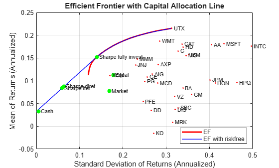
When a risk-free asset is not available to the portfolio, or in other words, the portfolio is fully invested, the efficient frontier is curved, corresponding to the red line in the above figure. Therefore, there is a unique (risk, return) point that maximizes the Sharpe ratio, which the 'iterative' and 'direct' methods will both find. If the portfolio is allowed to invest in a risk-free asset, part of the red efficient frontier line is replaced by the capital allocation line, resulting in the efficient frontier of a portfolio with a risk-free investment (blue line). All the (risk, return) points on the straight blue line share the same Sharpe ratio. Also, it is likely that the 'iterative' and 'direct' methods end up with different points, therefore there are different portfolio allocations.
When using the 'iterative' method, you can use an optional 'TolX' name-value argument. TolX is a termination tolerance that is related to the possible return levels of the efficient frontier. If the selected TolX value is large compared to the range of returns, then the accuracy of the solution is poor. TolX should be a number smaller than 0.01*(maxReturn - minReturn).
maxReturn = max(qret); % Max return portfolio
minReturn = min(qret); % Min return portfolio
display(0.01*(maxReturn-minReturn))
1.5192e-04
The purpose of increasing the termination tolerance is to speed up the convergence of the 'iterative' algorithm. However, as previously mentioned, the accuracy of the solution will decrease. You can see this in the table that follows.
pwgtshpr_iter_largerTol = estimateMaxSharpeRatio(q, 'Method', 'iterative',...
    'TolX', 1e-4);
display(table(pwgtshpr_iter, pwgtshpr_iter_largerTol,...
    'VariableNames', {'Default TolX = 1e-6','TolX = 1e-4'}))
  30×2 table

    Default TolX = 1e-6    TolX = 1e-4
    ___________________    ___________

        3.7125e-15          3.303e-16
         5.336e-15         4.2357e-16
         5.419e-15         3.3697e-16
         2.874e-15         2.3497e-16
        7.0895e-15           4.81e-16
        8.5366e-15         7.3441e-16
        1.6345e-15          1.374e-16
        2.2032e-15         1.9557e-16
        1.0796e-14         6.3893e-16
        3.6911e-15         2.6889e-16
        1.4772e-11         1.0431e-12
        1.6503e-15         1.3897e-16
        5.3201e-15         4.4754e-16
        4.8901e-15         9.2864e-16
          0.011343           0.012148
          0.038342           0.041063
        2.2056e-15         1.7203e-16
        1.6027e-15         1.2027e-16
        3.6314e-15         2.7911e-16
          0.066008           0.070692
          0.059598           0.063827
        1.9646e-15          1.531e-16
          0.019067            0.02042
        3.5371e-15         2.9318e-16
          0.031761           0.034014
        1.7433e-15         1.5431e-16
          0.025573           0.027387
        1.9441e-15         1.7488e-16
          0.093897            0.10056
          0.080228            0.08592
In the table, the value of the weights varies slightly with respect to the weights obtained with the default tolerance, as expected.
Create a Portfolio object for three assets.
AssetMean = [ 0.0101110; 0.0043532; 0.0137058 ];
AssetCovar = [ 0.00324625 0.00022983 0.00420395;
               0.00022983 0.00049937 0.00019247;
               0.00420395 0.00019247 0.00764097 ];
p = Portfolio('AssetMean', AssetMean, 'AssetCovar', AssetCovar);
p = setDefaultConstraints(p);
Use setBounds with semicontinuous constraints to set xi = 0 or 0.02 <= xi <= 0.5 for all i = 1,...NumAssets.
p = setBounds(p, 0.02, 0.5,'BoundType', 'Conditional', 'NumAssets', 3);
When working with a Portfolio object, the setMinMaxNumAssets function enables you to set up cardinality constraints for a long-only portfolio. This sets the cardinality constraints for the Portfolio object, where the total number of allocated assets satisfying the nonzero semi-continuous constraints are between MinNumAssets and MaxNumAssets. By setting MinNumAssets = MaxNumAssets = 2, only two of the three assets are invested in the portfolio.
p = setMinMaxNumAssets(p, 2, 2);
Use estimateMaxSharpeRatio to estimate efficient portfolio to maximize Sharpe ratio.
weights = estimateMaxSharpeRatio(p,'Method','iterative')
weights = 3×1

         0
    0.5000
    0.5000
The estimateMaxSharpeRatio function uses the MINLP solver to solve this problem. Use the setSolverMINLP function to configure the SolverType and options.
p.solverOptionsMINLP
ans = struct with fields:
                           MaxIterations: 1000
                    AbsoluteGapTolerance: 1.0000e-07
                    RelativeGapTolerance: 1.0000e-05
                  NonlinearScalingFactor: 1000
                  ObjectiveScalingFactor: 1000
                                 Display: 'off'
                           CutGeneration: 'basic'
                MaxIterationsInactiveCut: 15
                      ActiveCutTolerance: 1.0000e-07
                   CutSelectionHeuristic: 'quantile'
                       QuantileThreshold: 0.6000
                    IntMainSolverOptions: [1×1 optim.options.Intlinprog]
    NumIterationsEarlyIntegerConvergence: 30
                     ExtendedFormulation: 0
                            NumInnerCuts: 10
                     NumInitialOuterCuts: 10
Input Arguments
Name-Value Arguments
Output Arguments
More About
Tips
You can also use dot notation to estimate an efficient portfolio that maximizes the Sharpe ratio.
[pwgt,pbuy,psell] = obj.estimateMaxSharpeRatio;
Algorithms
The maximization of the Sharpe ratio is accomplished by either using the
'direct' or 'iterative'
method. For the 'direct' method, consider the following
scenario. To maximize the Sharpe ratio is to:
where μ and C are the mean and covariance matrix, and rf is the risk-free rate.
If μT x - rf ≤ 0 for all x the portfolio that maximizes the Sharpe ratio is the one with maximum return.
If μT x - rf > 0, let
and y = tx (Cornuejols [1] section 8.2). Then after some substitutions, you can transform the original problem into the following form,
Only one optimization needs to be solved, hence the name “direct”. The portfolio weights can be recovered by x* = y* / t*.
For the 'iterative' method, the idea is to iteratively
explore the portfolios at different return levels on the efficient frontier
and locate the one with maximum Sharpe ratio. Therefore, multiple
optimization problems are solved during the process, instead of only one in
the 'direct' method. Consequently, the
'iterative' method is slow compared to
'direct' method.
References
[1] Cornuejols, G. and Reha Tütüncü. Optimization Methods in Finance. Cambridge University Press, 2007.
Version History
Introduced in R2011bSee Also
estimatePortSharpeRatio | estimateFrontier | estimateFrontierByReturn | estimateFrontierByRisk | setBounds | setMinMaxNumAssets
Topics
- Estimate Efficient Portfolios for Entire Efficient Frontier for Portfolio Object
- Working with 'Conditional' BoundType, MinNumAssets, and MaxNumAssets Constraints Using Portfolio Objects
- Portfolio Optimization Examples Using Financial Toolbox
- Bond Portfolio Optimization Using Portfolio Object
- Portfolio Optimization Theory
- Choose MINLP Solvers for Portfolio Problems