estimateFrontier
Estimate specified number of optimal portfolios on the efficient frontier
Description
[ estimates the specified number of
optimal portfolios on the efficient frontier for pwgt,pbuy,psell]
= estimateFrontier(obj)Portfolio,
PortfolioCVaR, or PortfolioMAD objects. For details on
the respective workflows when using these different objects, see Portfolio Object Workflow, PortfolioCVaR Object Workflow, and PortfolioMAD Object Workflow.
Examples
Create efficient portfolios:
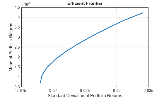
load CAPMuniverse

p = Portfolio('AssetList',Assets(1:12));
p = estimateAssetMoments(p, Data(:,1:12),'missingdata',true);
p = setDefaultConstraints(p);
plotFrontier(p);
pwgt = estimateFrontier(p, 5);

pnames = cell(1,5);
for i = 1:5
	pnames{i} = sprintf('Port%d',i);
end

Blotter = dataset([{pwgt},pnames],'obsnames',p.AssetList);

disp(Blotter);
            Port1         Port2         Port3         Port4         Port5
    AAPL      0.017926      0.058247      0.097816       0.12955    0
    AMZN     1.782e-13    1.5832e-11    2.1265e-10    2.0669e-11    0
    CSCO    1.3365e-14    7.4305e-13    5.1756e-11     2.798e-12    0
    DELL     0.0041906    4.0213e-10    2.9535e-09    1.0249e-10    0
    EBAY    1.2686e-14    1.6093e-12    1.0334e-10    1.0811e-11    0
    GOOG       0.16144       0.35678       0.55228       0.75116    1
    HPQ       0.052566      0.032302      0.011186    6.1882e-09    0
    IBM        0.46422       0.36045       0.25577       0.11928    0
    INTC    4.5883e-14    2.0534e-11     3.845e-08    1.8432e-08    0
    MSFT       0.29966       0.19222      0.082949    1.7512e-09    0
    ORCL    1.9196e-14    1.5317e-12    1.0064e-10    7.6664e-12    0
    YHOO    5.4342e-15    1.1905e-13    1.3146e-11    3.7126e-13    0
Create a Portfolio object for 12 stocks based on CAPMuniverse.mat.
load CAPMuniverse
p0 = Portfolio('AssetList',Assets(1:12));
p0 = estimateAssetMoments(p0, Data(:,1:12),'missingdata',true);
p0 = setDefaultConstraints(p0);
Use setMinMaxNumAssets to define a maximum number of 3 assets.
p1 = setMinMaxNumAssets(p0, [], 3);
Use setBounds to define a lower and upper bound and a BoundType of 'Conditional'.
p1 = setBounds(p1, 0.1, 0.5,'BoundType', 'Conditional');
pwgt = estimateFrontier(p1, 5);
The following table shows that the optimized allocations only have maximum 3 assets invested, and small positions less than 0.1 are avoided.
result = table(p0.AssetList', pwgt)
result=12×2 table
      Var1                             pwgt
    ________    ___________________________________________________

    {'AAPL'}          0          0          0    0.14232          0
    {'AMZN'}          0          0          0          0          0
    {'CSCO'}          0          0          0          0          0
    {'DELL'}          0          0          0          0          0
    {'EBAY'}          0          0          0          0        0.5
    {'GOOG'}    0.16891    0.29534    0.42177        0.5        0.5
    {'HPQ' }          0          0          0          0          0
    {'IBM' }    0.49968    0.43657    0.37326    0.35768          0
    {'INTC'}          0          0          0          0          0
    {'MSFT'}     0.3314     0.2681    0.20496          0          0
    {'ORCL'}          0          0          0          0          0
    {'YHOO'}          0          0          0          0          0
The estimateFrontier function uses the MINLP solver to solve this problem. Use the setSolverMINLP function to configure the SolverType and options.
p1.solverTypeMINLP
ans =
'OuterApproximation'
p1.solverOptionsMINLP
ans = struct with fields:
                           MaxIterations: 1000
                    AbsoluteGapTolerance: 1.0000e-07
                    RelativeGapTolerance: 1.0000e-05
                  NonlinearScalingFactor: 1000
                  ObjectiveScalingFactor: 1000
                                 Display: 'off'
                           CutGeneration: 'basic'
                MaxIterationsInactiveCut: 15
                      ActiveCutTolerance: 1.0000e-07
                   CutSelectionHeuristic: 'quantile'
                       QuantileThreshold: 0.6000
                    IntMainSolverOptions: [1×1 optim.options.Intlinprog]
    NumIterationsEarlyIntegerConvergence: 30
                     ExtendedFormulation: 0
                            NumInnerCuts: 10
                     NumInitialOuterCuts: 10
Create efficient portfolios:
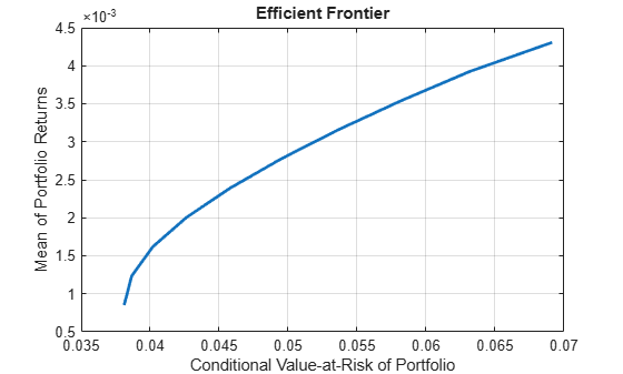
load CAPMuniverse

p = PortfolioCVaR('AssetList',Assets(1:12));
p = simulateNormalScenariosByData(p, Data(:,1:12), 20000 ,'missingdata',true);
p = setDefaultConstraints(p);
p = setProbabilityLevel(p, 0.95);

plotFrontier(p);
pwgt = estimateFrontier(p, 5);

pnames = cell(1,5);
for i = 1:5
	pnames{i} = sprintf('Port%d',i);
end

Blotter = dataset([{pwgt},pnames],'obsnames',p.AssetList);

disp(Blotter);
            Port1       Port2       Port3       Port4      Port5
    AAPL    0.010223    0.073393     0.11939    0.13137    0
    AMZN           0           0           0          0    0
    CSCO           0           0           0          0    0
    DELL     0.02301           0           0          0    0
    EBAY           0           0           0          0    0
    GOOG     0.20389     0.38068     0.56253    0.75919    1
    HPQ     0.041396    0.009472           0          0    0
    IBM      0.44369     0.36472     0.26247    0.10944    0
    INTC           0           0           0          0    0
    MSFT     0.27779     0.17174    0.055611          0    0
    ORCL           0           0           0          0    0
    YHOO           0           0           0          0    0
Create efficient portfolios:
load CAPMuniverse

p = PortfolioMAD('AssetList',Assets(1:12));
p = simulateNormalScenariosByData(p, Data(:,1:12), 20000 ,'missingdata',true);
p = setDefaultConstraints(p);

plotFrontier(p);

pwgt = estimateFrontier(p, 5);

pnames = cell(1,5);
for i = 1:5
	pnames{i} = sprintf('Port%d',i);
end

Blotter = dataset([{pwgt},pnames],'obsnames',p.AssetList);

disp(Blotter);
            Port1        Port2       Port3       Port4      Port5
    AAPL     0.029643    0.075874     0.11335    0.13405    0
    AMZN            0           0           0          0    0
    CSCO            0           0           0          0    0
    DELL    0.0086367           0           0          0    0
    EBAY            0           0           0          0    0
    GOOG      0.16177     0.35217     0.54489    0.74913    1
    HPQ      0.056891    0.023419           0          0    0
    IBM       0.45916     0.37921     0.29376    0.11682    0
    INTC            0           0           0          0    0
    MSFT       0.2839     0.16933    0.048005          0    0
    ORCL            0           0           0          0    0
    YHOO            0           0           0          0    0
Obtain the default number of efficient portfolios over the entire range of the efficient frontier.
m = [ 0.05; 0.1; 0.12; 0.18 ];
C = [ 0.0064 0.00408 0.00192 0;
    0.00408 0.0289 0.0204 0.0119;
    0.00192 0.0204 0.0576 0.0336;
    0 0.0119 0.0336 0.1225 ];

p = Portfolio;
p = setAssetMoments(p, m, C);
p = setDefaultConstraints(p);
pwgt = estimateFrontier(p);
disp(pwgt);
0.8891 0.7215 0.5540 0.3865 0.2190 0.0515 0.0000 0.0000 0.0000 0
0.0369 0.1289 0.2209 0.3129 0.4049 0.4969 0.4049 0.2314 0.0579 0
0.0404 0.0567 0.0730 0.0893 0.1056 0.1219 0.1320 0.1394 0.1468 0
0.0336 0.0929 0.1521 0.2113 0.2705 0.3297 0.4630 0.6292 0.7953 1.0000
Starting from the initial portfolio, the estimateFrontier function returns purchases and sales to get from your initial portfolio to each efficient portfolio on the efficient frontier. Given an initial portfolio in pwgt0, you can obtain purchases and sales.
m = [ 0.05; 0.1; 0.12; 0.18 ];
C = [ 0.0064 0.00408 0.00192 0;
0.00408 0.0289 0.0204 0.0119;
0.00192 0.0204 0.0576 0.0336;
0 0.0119 0.0336 0.1225 ];
p = Portfolio;
p = setAssetMoments(p, m, C);
p = setDefaultConstraints(p);
pwgt0 = [ 0.3; 0.3; 0.2; 0.1 ];
p = setInitPort(p, pwgt0);
[pwgt, pbuy, psell] = estimateFrontier(p);
display(pwgt);pwgt = 4×10
    0.8891    0.7215    0.5540    0.3865    0.2190    0.0515    0.0000    0.0000    0.0000         0
    0.0369    0.1289    0.2209    0.3129    0.4049    0.4969    0.4049    0.2314    0.0579         0
    0.0404    0.0567    0.0730    0.0893    0.1056    0.1219    0.1320    0.1394    0.1468         0
    0.0336    0.0929    0.1521    0.2113    0.2705    0.3297    0.4630    0.6292    0.7953    1.0000
display(pbuy);
pbuy = 4×10

    0.5891    0.4215    0.2540    0.0865         0         0         0         0         0         0
         0         0         0    0.0129    0.1049    0.1969    0.1049         0         0         0
         0         0         0         0         0         0         0         0         0         0
         0         0    0.0521    0.1113    0.1705    0.2297    0.3630    0.5292    0.6953    0.9000
display(psell);
psell = 4×10

         0         0         0         0    0.0810    0.2485    0.3000    0.3000    0.3000    0.3000
    0.2631    0.1711    0.0791         0         0         0         0    0.0686    0.2421    0.3000
    0.1596    0.1433    0.1270    0.1107    0.0944    0.0781    0.0680    0.0606    0.0532    0.2000
    0.0664    0.0071         0         0         0         0         0         0         0         0
Obtain the default number of efficient portfolios over the entire range of the efficient frontier.
m = [ 0.05; 0.1; 0.12; 0.18 ];
C = [ 0.0064 0.00408 0.00192 0;
    0.00408 0.0289 0.0204 0.0119;
    0.00192 0.0204 0.0576 0.0336;
    0 0.0119 0.0336 0.1225 ];
m = m/12;
C = C/12;

rng(11);

AssetScenarios = mvnrnd(m, C, 20000);

p = PortfolioCVaR;
p = setScenarios(p, AssetScenarios);
p = setDefaultConstraints(p);
p = setProbabilityLevel(p, 0.95);

pwgt = estimateFrontier(p);

disp(pwgt);
0.8445 0.6841 0.5148 0.3534 0.1897 0.0303 0 0 0 0
0.0609 0.1429 0.2302 0.3171 0.3987 0.4742 0.3524 0.1803 0 0
0.0458 0.0640 0.0945 0.1081 0.1340 0.1590 0.1738 0.1918 0.2211 0
0.0488 0.1090 0.1606 0.2215 0.2776 0.3365 0.4738 0.6280 0.7789 1.0000
The function rng() resets the random number generator to produce the documented results. It is not necessary to reset the random number generator to simulate scenarios.
Starting from the initial portfolio, the estimateFrontier function returns purchases and sales to get from your initial portfolio to each efficient portfolio on the efficient frontier. Given an initial portfolio in pwgt0, you can obtain purchases and sales.
m = [ 0.05; 0.1; 0.12; 0.18 ];
C = [ 0.0064 0.00408 0.00192 0;
0.00408 0.0289 0.0204 0.0119;
0.00192 0.0204 0.0576 0.0336;
0 0.0119 0.0336 0.1225 ];
m = m/12;
C = C/12;
rng(11);
AssetScenarios = mvnrnd(m, C, 20000);
p = PortfolioCVaR;
p = setScenarios(p, AssetScenarios);
p = setDefaultConstraints(p);
p = setProbabilityLevel(p, 0.95);
pwgt0 = [ 0.3; 0.3; 0.2; 0.1 ];
p = setInitPort(p, pwgt0);
[pwgt, pbuy, psell] = estimateFrontier(p);
display(pwgt);pwgt = 4×10
    0.8445    0.6841    0.5148    0.3534    0.1897    0.0303         0         0         0         0
    0.0609    0.1429    0.2302    0.3171    0.3987    0.4742    0.3524    0.1803         0         0
    0.0458    0.0640    0.0945    0.1081    0.1340    0.1590    0.1738    0.1918    0.2211         0
    0.0488    0.1090    0.1606    0.2215    0.2776    0.3365    0.4738    0.6280    0.7789    1.0000
display(pbuy);
pbuy = 4×10

    0.5445    0.3841    0.2148    0.0534         0         0         0         0         0         0
         0         0         0    0.0171    0.0987    0.1742    0.0524         0         0         0
         0         0         0         0         0         0         0         0    0.0211         0
         0    0.0090    0.0606    0.1215    0.1776    0.2365    0.3738    0.5280    0.6789    0.9000
display(psell);
psell = 4×10

         0         0         0         0    0.1103    0.2697    0.3000    0.3000    0.3000    0.3000
    0.2391    0.1571    0.0698         0         0         0         0    0.1197    0.3000    0.3000
    0.1542    0.1360    0.1055    0.0919    0.0660    0.0410    0.0262    0.0082         0    0.2000
    0.0512         0         0         0         0         0         0         0         0         0
The function rng() resets the random number generator to produce the documented results. It is not necessary to reset the random number generator to simulate scenarios.
Obtain the default number of efficient portfolios over the entire range of the efficient frontier.
m = [ 0.05; 0.1; 0.12; 0.18 ];
C = [ 0.0064 0.00408 0.00192 0;
    0.00408 0.0289 0.0204 0.0119;
    0.00192 0.0204 0.0576 0.0336;
    0 0.0119 0.0336 0.1225 ];
m = m/12;
C = C/12;

rng(11);

AssetScenarios = mvnrnd(m, C, 20000);

p = PortfolioMAD;
p = setScenarios(p, AssetScenarios);
p = setDefaultConstraints(p);

pwgt = estimateFrontier(p);

disp(pwgt);
0.8817 0.7150 0.5488 0.3811 0.2173 0.0503 0 0 0 0
0.0435 0.1290 0.2130 0.2987 0.3821 0.4668 0.3614 0.1751 0 0
0.0385 0.0600 0.0826 0.1061 0.1242 0.1477 0.1780 0.2101 0.2267 0
0.0363 0.0960 0.1556 0.2141 0.2764 0.3352 0.4605 0.6148 0.7733 1.0000
The function rng() resets the random number generator to produce the documented results. It is not necessary to reset the random number generator to simulate scenarios.
Starting from the initial portfolio, the estimateFrontier function returns purchases and sales to get from your initial portfolio to each efficient portfolio on the efficient frontier. Given an initial portfolio in pwgt0, you can obtain purchases and sales.
m = [ 0.05; 0.1; 0.12; 0.18 ];
C = [ 0.0064 0.00408 0.00192 0;
0.00408 0.0289 0.0204 0.0119;
0.00192 0.0204 0.0576 0.0336;
0 0.0119 0.0336 0.1225 ];
m = m/12;
C = C/12;
rng(11);
AssetScenarios = mvnrnd(m, C, 20000);
p = PortfolioMAD;
p = setScenarios(p, AssetScenarios);
p = setDefaultConstraints(p);
pwgt0 = [ 0.3; 0.3; 0.2; 0.1 ];
p = setInitPort(p, pwgt0);
[pwgt, pbuy, psell] = estimateFrontier(p);
display(pwgt);pwgt = 4×10
    0.8817    0.7150    0.5488    0.3811    0.2173    0.0503         0         0         0         0
    0.0435    0.1290    0.2130    0.2987    0.3821    0.4668    0.3614    0.1751         0         0
    0.0385    0.0600    0.0826    0.1061    0.1242    0.1477    0.1780    0.2101    0.2267         0
    0.0363    0.0960    0.1556    0.2141    0.2764    0.3352    0.4605    0.6148    0.7733    1.0000
display(pbuy);
pbuy = 4×10

    0.5817    0.4150    0.2488    0.0811         0         0         0         0         0         0
         0         0         0         0    0.0821    0.1668    0.0614         0         0         0
         0         0         0         0         0         0         0    0.0101    0.0267         0
         0         0    0.0556    0.1141    0.1764    0.2352    0.3605    0.5148    0.6733    0.9000
display(psell);
psell = 4×10

         0         0         0         0    0.0827    0.2497    0.3000    0.3000    0.3000    0.3000
    0.2565    0.1710    0.0870    0.0013         0         0         0    0.1249    0.3000    0.3000
    0.1615    0.1400    0.1174    0.0939    0.0758    0.0523    0.0220         0         0    0.2000
    0.0637    0.0040         0         0         0         0         0         0         0         0
The function rng() resets the random number generator to produce the documented results. It is not necessary to reset the random number generator to simulate scenarios.
Input Arguments
Output Arguments
More About
Tips
You can also use dot notation to estimate the specified number of optimal portfolios over the entire efficient frontier.
[pwgt, pbuy, psell] = obj.estimateFrontier(NumPorts);
When introducing transaction costs and turnover constraints to the
Portfolio,PortfolioCVaR, orPortfolioMADobject, the portfolio optimization objective contains a term with an absolute value. For more information on how Financial Toolbox™ handles such cases algorithmically, see References.
References
[1] Cornuejols, G., and R. Tutuncu. Optimization Methods in Finance. Cambridge University Press, 2007.
Version History
Introduced in R2011a
See Also
estimateFrontierByReturn | estimateFrontierByRisk | estimateFrontierLimits | setBounds | setMinMaxNumAssets
Topics
- Estimate Efficient Portfolios for Entire Efficient Frontier for Portfolio Object
- Estimate Efficient Frontiers for Portfolio Object
- Estimate Efficient Portfolios for Entire Frontier for PortfolioCVaR Object
- Estimate Efficient Frontiers for PortfolioCVaR Object
- Estimate Efficient Portfolios Along the Entire Frontier for PortfolioMAD Object
- Estimate Efficient Frontiers for PortfolioMAD Object
- Portfolio Optimization Examples Using Financial Toolbox
- Bond Portfolio Optimization Using Portfolio Object
- Portfolio Optimization Theory
- Choose MINLP Solvers for Portfolio Problems