Main Content

setSolverMINLP

Choose mixed integer nonlinear programming (MINLP) solver for portfolio optimization

Description

example

obj = setSolverMINLP(obj,solverTypeMINLP) selects the mixed integer nonlinear programming (MINLP) solver and enables you to specify associated solver options for portfolio optimization for a Portfolio, PortfolioCVaR, or PortfolioMAD object.

When any one or any combination of 'Conditional' BoundType, MinNumAssets, or MaxNumAssets constraints are active, the portfolio problem is formulated by adding NumAssets binary variables. The binary variable 0 indicates that an asset is not invested and the binary variable 1 indicates that an asset is invested. For more information on using 'Conditional' BoundType, see setBounds. For more information on specifying MinNumAssets and MaxNumAssets, see setMinMaxNumAssets.

If you use the Financial Toolbox™ estimate functions with a Portfolio, PortfolioCVaR, or PortfolioMAD object for which any of the 'Conditional' BoundType, MinNumAssets, or MaxNumAssets constraints are active, MINLP solver is automatically used. For details on MINLP, see Algorithms and Choose MINLP Solvers for Portfolio Problems.

example

obj = setSolverMINLP(___,Name,Value) specifies options using one or more name-value arguments in addition to the input arguments in the previous syntax.

Examples

collapse all

Configure the MINLP solver for a three-asset portfolio for which you have the mean and covariance values of the asset returns.

AssetMean = [ 0.0101110; 0.0043532; 0.0137058 ];
AssetCovar = [ 0.00324625 0.00022983 0.00420395;
               0.00022983 0.00049937 0.00019247;
               0.00420395 0.00019247 0.00764097 ]; 
p = Portfolio('AssetMean', AssetMean, 'AssetCovar', AssetCovar);

When working with a Portfolio object, use setBounds with a 'Conditional'BoundType constraint to set xi = 0 or 0.02 <= xi <= 0.5 for all i = 1,...NumAssets.

p = setBounds(p, 0.02, 0.5,'BoundType', 'Conditional', 'NumAssets', 3); 

When working with a Portfolio object, use setMinMaxNumAssets function to set up MinNumAssets and MaxNumAssets constraints for a portfolio. This sets limit constraints for the Portfolio object, where the total number of allocated assets satisfying the constraints is between MinNumAssets and MaxNumAssets. Setting MinNumAssets = MaxNumAssets = 2, specifies that only two of the three assets are invested in the portfolio.

p = setMinMaxNumAssets(p, 2, 2); 

Three different MINLP solvers (OuterApproximation, ExtendedCP, TrustRegionCP) use the cutting plane method. Use the setSolverMINLP function to configure the OuterApproximation solver and options.

pint = setSolverMINLP(p,'OuterApproximation', 'NonlinearScalingFactor', 1e4, 'Display', 'iter', 'CutGeneration', 'basic');
pint.solverTypeMINLP
ans = 
'OuterApproximation'
pint.solverOptionsMINLP
ans = struct with fields:
                           MaxIterations: 1000
                    AbsoluteGapTolerance: 1.0000e-07
                    RelativeGapTolerance: 1.0000e-05
                  NonlinearScalingFactor: 10000
                  ObjectiveScalingFactor: 1000
                                 Display: 'iter'
                           CutGeneration: 'basic'
                MaxIterationsInactiveCut: 30
                      ActiveCutTolerance: 1.0000e-07
                    IntMainSolverOptions: [1x1 optim.options.Intlinprog]
    NumIterationsEarlyIntegerConvergence: 30
                     ExtendedFormulation: 0
                            NumInnerCuts: 10
                     NumInitialOuterCuts: 10

You can also configure the options for intlinprog, which is the Main solver for mixed integer linear programming problems in the MINLP solver.

pint = setSolverMINLP(p,'OuterApproximation', 'IntMainSolverOptions', optimoptions('intlinprog','Display','off'));
pint.solverOptionsMINLP.IntMainSolverOptions
ans = 
  intlinprog options:

   Set properties:
                          Display: 'off'

   Default properties:
             AbsoluteGapTolerance: 0
                       BranchRule: 'reliability'
              ConstraintTolerance: 1.0000e-04
                    CutGeneration: 'basic'
                 CutMaxIterations: 10
                       Heuristics: 'basic'
               HeuristicsMaxNodes: 50
                IntegerPreprocess: 'basic'
                 IntegerTolerance: 1.0000e-05
                  LPMaxIterations: 'max(30000,10*(numberOfEqualities+numberOfInequalities+numberOfVariables))'
            LPOptimalityTolerance: 1.0000e-07
                MaxFeasiblePoints: Inf
                         MaxNodes: 10000000
                          MaxTime: 7200
                    NodeSelection: 'simplebestproj'
                  ObjectiveCutOff: Inf
    ObjectiveImprovementThreshold: 0
                        OutputFcn: []
                          PlotFcn: []
             RelativeGapTolerance: 1.0000e-04
                  RootLPAlgorithm: 'dual-simplex'
              RootLPMaxIterations: 'max(30000,10*(numberOfEqualities+numberOfInequalities+numberOfVariables))'

Configure the MINLP solver for a 12 asset portfolio that is using semicontinuous and cardinality constraints.

load CAPMuniverse
p = PortfolioCVaR('AssetList',Assets(1:12));
p = simulateNormalScenariosByData(p, Data(:,1:12),20000,'missingdata',true);
p = setProbabilityLevel(p, 0.95);

When working with a PortfolioCVaR object, the setMinMaxNumAssets function enables you to set up the limits on the number of assets invested. The following example specifies that a minimum of five assets and a maximum of 10 assets should be invested using setMinMaxNumAssets and the investments should be greater than 4% and less than 45% using setBounds.

p = setMinMaxNumAssets(p, 5, 10);  
p = setBounds(p, 0.04, 0.45, 'BoundType','conditional');  

Three different MINLP solvers (OuterApproximation, ExtendedCP, TrustRegionCP) use the cutting plane method. Use the setSolverMINLP function to configure the OuterApproximation solver and options.

pint = setSolverMINLP(p,'OuterApproximation','NonlinearScalingFactor', 1e4, 'Display', 'iter', 'CutGeneration', 'basic');
pint.solverTypeMINLP
ans = 
'OuterApproximation'
pint.solverOptionsMINLP
ans = struct with fields:
                           MaxIterations: 1000
                    AbsoluteGapTolerance: 1.0000e-07
                    RelativeGapTolerance: 1.0000e-05
                  NonlinearScalingFactor: 10000
                  ObjectiveScalingFactor: 1000
                                 Display: 'iter'
                           CutGeneration: 'basic'
                MaxIterationsInactiveCut: 30
                      ActiveCutTolerance: 1.0000e-07
                    IntMainSolverOptions: [1x1 optim.options.Intlinprog]
    NumIterationsEarlyIntegerConvergence: 30
                     ExtendedFormulation: 0
                            NumInnerCuts: 10
                     NumInitialOuterCuts: 10

You can also configure the options for intlinprog, which is the Main solver for mixed integer linear programming problems in the MINLP solver.

pint = setSolverMINLP(p,'OuterApproximation','IntMainSolverOptions', optimoptions('intlinprog','Display','off'));
pint.solverOptionsMINLP.IntMainSolverOptions
ans = 
  intlinprog options:

   Set properties:
                          Display: 'off'

   Default properties:
             AbsoluteGapTolerance: 0
                       BranchRule: 'reliability'
              ConstraintTolerance: 1.0000e-04
                    CutGeneration: 'basic'
                 CutMaxIterations: 10
                       Heuristics: 'basic'
               HeuristicsMaxNodes: 50
                IntegerPreprocess: 'basic'
                 IntegerTolerance: 1.0000e-05
                  LPMaxIterations: 'max(30000,10*(numberOfEqualities+numberOfInequalities+numberOfVariables))'
            LPOptimalityTolerance: 1.0000e-07
                MaxFeasiblePoints: Inf
                         MaxNodes: 10000000
                          MaxTime: 7200
                    NodeSelection: 'simplebestproj'
                  ObjectiveCutOff: Inf
    ObjectiveImprovementThreshold: 0
                        OutputFcn: []
                          PlotFcn: []
             RelativeGapTolerance: 1.0000e-04
                  RootLPAlgorithm: 'dual-simplex'
              RootLPMaxIterations: 'max(30000,10*(numberOfEqualities+numberOfInequalities+numberOfVariables))'

Configure the MINLP solver for a 12 asset portfolio that is using semicontinuous and cardinality constraints.

load CAPMuniverse
p = PortfolioMAD('AssetList',Assets(1:12));
p = simulateNormalScenariosByData(p, Data(:,1:12), 20000 ,'missingdata',true);

When working with a PortfolioMAD object, the setMinMaxNumAssets function enables you to set up the limits on the number of assets invested. The following example specifies that a minimum of five assets and a maximum of 10 assets should be invested using setMinMaxNumAssets and the investments should be greater than 4% and less than 45% using setBounds.

p = setMinMaxNumAssets(p, 5, 10);  
p = setBounds(p, 0.04, 0.45, 'BoundType', 'conditional');  

Three different MINLP solvers (OuterApproximation, ExtendedCP, TrustRegionCP) use the cutting plane method. Use the setSolverMINLP function to configure the OuterApproximation solver and options.

pint = setSolverMINLP(p,'OuterApproximation', 'NonlinearScalingFactor', 1e4, 'Display', 'iter', 'CutGeneration', 'basic');
pint.solverTypeMINLP
ans = 
'OuterApproximation'
pint.solverOptionsMINLP
ans = struct with fields:
                           MaxIterations: 1000
                    AbsoluteGapTolerance: 1.0000e-07
                    RelativeGapTolerance: 1.0000e-05
                  NonlinearScalingFactor: 10000
                  ObjectiveScalingFactor: 1000
                                 Display: 'iter'
                           CutGeneration: 'basic'
                MaxIterationsInactiveCut: 30
                      ActiveCutTolerance: 1.0000e-07
                    IntMainSolverOptions: [1x1 optim.options.Intlinprog]
    NumIterationsEarlyIntegerConvergence: 30
                     ExtendedFormulation: 0
                            NumInnerCuts: 10
                     NumInitialOuterCuts: 10

You can also configure the options for intlinprog, which is the Main solver for mixed integer linear programming problems in the MINLP solver.

pint = setSolverMINLP(p,'OuterApproximation', 'IntMainSolverOptions', optimoptions('intlinprog','Display','off'));
pint.solverOptionsMINLP.IntMainSolverOptions
ans = 
  intlinprog options:

   Set properties:
                          Display: 'off'

   Default properties:
             AbsoluteGapTolerance: 0
                       BranchRule: 'reliability'
              ConstraintTolerance: 1.0000e-04
                    CutGeneration: 'basic'
                 CutMaxIterations: 10
                       Heuristics: 'basic'
               HeuristicsMaxNodes: 50
                IntegerPreprocess: 'basic'
                 IntegerTolerance: 1.0000e-05
                  LPMaxIterations: 'max(30000,10*(numberOfEqualities+numberOfInequalities+numberOfVariables))'
            LPOptimalityTolerance: 1.0000e-07
                MaxFeasiblePoints: Inf
                         MaxNodes: 10000000
                          MaxTime: 7200
                    NodeSelection: 'simplebestproj'
                  ObjectiveCutOff: Inf
    ObjectiveImprovementThreshold: 0
                        OutputFcn: []
                          PlotFcn: []
             RelativeGapTolerance: 1.0000e-04
                  RootLPAlgorithm: 'dual-simplex'
              RootLPMaxIterations: 'max(30000,10*(numberOfEqualities+numberOfInequalities+numberOfVariables))'

This example shows how to solve a portfolio optimization problem with constraints in the number of selected assets and conditional (semi-continuous) bounds. This example demonstrates setSolverMINLP support for extended formulation, using the name-value argument ExtendedFormulation, for the OuterApproximation solverTypeMINLP. The extended formulation reformulates problems with quadratic functions to work in an extended space to decrease the computation time.

Create Mean-Variance Portfolio

Load the returns data in CAPMuniverse.mat. Then, create a standard mean-variance Portfolio object with default constraints, a long-only portfolio whose weights sum to 1. For this example, you can define the feasible region of weights X as

X={x|i=1nxi=1,xi0}.

% Load data
load CAPMuniverse.mat

% Create a mean-variance Portfolio object with default constraints
p = Portfolio(AssetList=Assets(1:12));
p = estimateAssetMoments(p,Data(:,1:12));
p = setDefaultConstraints(p);
p.solverOptionsMINLP
ans = struct with fields:
                           MaxIterations: 1000
                    AbsoluteGapTolerance: 1.0000e-07
                    RelativeGapTolerance: 1.0000e-05
                  NonlinearScalingFactor: 1000
                  ObjectiveScalingFactor: 1000
                                 Display: 'off'
                           CutGeneration: 'basic'
                MaxIterationsInactiveCut: 30
                      ActiveCutTolerance: 1.0000e-07
                    IntMainSolverOptions: [1x1 optim.options.Intlinprog]
    NumIterationsEarlyIntegerConvergence: 30
                     ExtendedFormulation: 0
                            NumInnerCuts: 10
                     NumInitialOuterCuts: 10

Include binary variables for this scenario by setting conditional (semicontinuous) bounds using setBounds. Conditional bounds are those such that xi=0 or xii. In this example, i=0.1 for all assets.

% Set conditional bounds
condLB = 0.1;
condUB = 0.5;
p = setBounds(p,condLB,condUB,BoundType="conditional")
p = 
  Portfolio with properties:

          BuyCost: []
         SellCost: []
     RiskFreeRate: []
        AssetMean: [12x1 double]
       AssetCovar: [12x12 double]
    TrackingError: []
     TrackingPort: []
         Turnover: []
      BuyTurnover: []
     SellTurnover: []
             Name: []
        NumAssets: 12
        AssetList: {'AAPL'  'AMZN'  'CSCO'  'DELL'  'EBAY'  'GOOG'  'HPQ'  'IBM'  'INTC'  'MSFT'  'ORCL'  'YHOO'}
         InitPort: []
      AInequality: []
      bInequality: []
        AEquality: []
        bEquality: []
       LowerBound: [12x1 double]
       UpperBound: [12x1 double]
      LowerBudget: 1
      UpperBudget: 1
      GroupMatrix: []
       LowerGroup: []
       UpperGroup: []
           GroupA: []
           GroupB: []
       LowerRatio: []
       UpperRatio: []
     MinNumAssets: []
     MaxNumAssets: []
        BoundType: [12x1 categorical]

Set ExtendedFormulation of OuterApproximation

Use setSolverMINLP to apply the extended formulation to the problem by setting the solverTypeMINLP argument for OuterApproximation and the ExtendedFromulation name-value argument to true. The extended formulation reformulates problems with quadratic functions to work in an extended space to decrease the computation time. You can use the name-value arguments NumInnerCuts and NumInitialOuterCuts to control the extended formulation algorithm:

  • NumInnerCuts — Number of cuts per asset added to the inner approximation problem to obtain an initial feasible point and upper bound

  • NumInitialOuterCuts — Number of cuts per asset added to the initial outer approximation problem.

% Increase the number of inner cuts and intial outer cuts
pEOA = setSolverMINLP(p,'OuterApproximation',ExtendedFormulation=true,NumInnerCuts=20,NumInitialOuterCuts=20);
pEOA.solverOptionsMINLP 
ans = struct with fields:
                           MaxIterations: 1000
                    AbsoluteGapTolerance: 1.0000e-07
                    RelativeGapTolerance: 1.0000e-05
                  NonlinearScalingFactor: 1000
                  ObjectiveScalingFactor: 1000
                                 Display: 'off'
                           CutGeneration: 'basic'
                MaxIterationsInactiveCut: 30
                      ActiveCutTolerance: 1.0000e-07
                    IntMainSolverOptions: [1x1 optim.options.Intlinprog]
    NumIterationsEarlyIntegerConvergence: 30
                     ExtendedFormulation: 1
                            NumInnerCuts: 20
                     NumInitialOuterCuts: 20

Estimate Set of Portfolios on Efficient Frontier

Use estimateFrontier to compute the efficient frontier, which is the curve that shows the trade-off between the return and risk achieved by Pareto-optimal portfolios. For a given return level, the portfolio on the efficient frontier is the one that minimizes the risk while maintaining the desired return. Conversely, for a given risk level, the portfolio on the efficient frontier is the one that maximizes return while maintaining the desired risk level. Compute risks and returns of the portfolios on the efficient frontier.

% Find the efficient frontier
wEOA = estimateFrontier(pEOA)
wEOA = 12×10

         0         0    0.1000    0.1253    0.1745    0.2236    0.2715    0.3327    0.4111    0.5000
         0         0         0         0         0         0         0         0         0         0
         0         0         0         0         0         0         0         0         0         0
    0.1350         0         0         0         0         0         0         0         0         0
         0         0         0         0         0         0         0         0         0         0
    0.1000    0.1450    0.1406    0.1910    0.2344    0.2778    0.3200    0.3726    0.4415    0.5000
    0.1000    0.1609    0.1642    0.2121    0.2415    0.2709    0.3085    0.2947    0.1474         0
    0.2354    0.1875    0.1290         0         0         0         0         0         0         0
         0         0         0         0         0         0         0         0         0         0
    0.4296    0.4066    0.3662    0.3717    0.2496    0.1277         0         0         0         0
      ⋮

% Compute risk and returns of the portfolios on the efficient frontier
[rskEOA,retEOA] = estimatePortMoments(p,wEOA)
rskEOA = 10×1

    0.0076
    0.0080
    0.0085
    0.0094
    0.0105
    0.0117
    0.0132
    0.0147
    0.0168
    0.0193

retEOA = 10×1

    0.0008
    0.0012
    0.0017
    0.0021
    0.0026
    0.0030
    0.0034
    0.0039
    0.0043
    0.0048

Maximize Return By Risk

Problems modeled to obtain the efficient frontier are of the type that minimizes risk subject to a return level. Another common portfolio problem is one that maximizes return for a fixed risk level. The risk level selected should be achievable by the portfolio. That is, the risk level should be between the risk attained by the minimum risk portfolio and the maximum return portfolio. The following code first checks if the target risk level is achievable and, if it is, computes the portfolio that maximizes the return subject to the target risk level.

% Set a risk level that is "achievable"
targetRisk_A = mean(rskEOA);
wAchievRisk = estimateFrontierByRisk(p,targetRisk_A)
wAchievRisk = 12×1

    0.2322
         0
    0.0000
         0
         0
    0.2853
    0.2760
    0.0000
    0.0000
    0.1065
      ⋮

Input Arguments

collapse all

Object for portfolio, specified using Portfolio, PortfolioCVaR, or PortfolioMAD object. For more information on creating a portfolio object, see

Data Types: object

MINLP solver for portfolio optimization when any one or any combination of 'Conditional' BoundType, MinNumAssets, or MaxNumAssets constraints are active. Specify solverTypeMINLP using a character vector or string with a value of 'OuterApproximation', or 'ExtendedCP', 'TrustRegionCP'.

Using Portfolio Object

Using PortfolioCVaR or PortfolioMAD Object

For a PortfolioCVaR and PortfolioMAD object, the default value of the solverTypeMINLP is 'TrustRegionCP' with the following default settings for name-value pairs for setSolverMINLP:

  • MaxIterations1000

  • AbsoluteGapTolerance1.0000e-07

  • RelativeGapTolerance1.0000e-05

  • Display'off'

  • NonlinearScalingFactor1000

  • ObjectiveScalingFactor1000

  • CutGeneration'basic'

  • MaxIterationsInactiveCut30

  • NumIterationsEarlyIntegerConvergence30

  • ActiveCutTolerance1.0000e-07

  • TrustRegionStartIteration - 2

  • ShrinkRatio0.75

  • InitialDelta0.5

  • DeltaLimit1e6

  • DeltaLowerBound0.01

  • IntMainSolverOptionsoptimoptions('intlinprog','Algorithm','Dual-Simplex','Display','off')

Data Types: char | string

Name-Value Arguments

Specify optional pairs of arguments as Name1=Value1,...,NameN=ValueN, where Name is the argument name and Value is the corresponding value. Name-value arguments must appear after other arguments, but the order of the pairs does not matter.

Before R2021a, use commas to separate each name and value, and enclose Name in quotes.

Example: p = setSolverMINLP(p,'ExtendedCP','MaxIterations',10000,'NonlinearScalingFactor',1000)

Maximum number of iterations, specified as the comma-separated pair consisting of 'MaxIterations' and a nonnegative integer value.

Data Types: double

Scaling factor for nonlinear function and gradient, specified as the comma-separated pair consisting of 'NonlinearScalingFactor' and a nonnegative real value.

Data Types: double

Scales the objective function used by MainSolver by a factor, specified as the comma-separated pair consisting of 'ObjectiveScalingFactor' and a nonnegative real value.

Data Types: double

The solver stops if the absolute difference between the approximated nonlinear function value and its true value is less than or equal to AbsoluteGapTolerance. AbsoluteGapTolerance is specified as the comma-separated pair consisting of 'AbsoluteGapTolerance' and a nonnegative real value.

Data Types: double

The solver stops if the relative difference between the approximated nonlinear function value and its true value is less than or equal to RelativeGapTolerance. RelativeGapTolerance is specified as the comma-separated pair consisting of 'AbsoluteGapTolerance' and a nonnegative real value.

Data Types: double

Display output format, specified as the comma-separated pair consisting of 'Display' and a character vector with a value of:

  • 'off' — Display no output

  • 'iter' — Display output at each iteration and the technical exit message

  • 'final' — Display only the final output and the final technical exit message

Data Types: char

Cut specification, specified as the comma-separated pair consisting of 'CutGeneration' and a character vector with one of these values:

  • 'basic' — Add the new cut at the latest solution found.

  • 'midway' — Add the new cut at the midpoint between the latest and previous solutions found.

Data Types: char

Since R2023b

Extend problem if all functions are linear or quadratic for a Portfolio object, specified as the comma-separated pair consisting of 'ExtendedFormulation' and a logical value:

  • true — If possible, use extended formulation. When set to true, you can specify a value for NumInnerCuts and NumInitialOuterCuts.

  • false — Use original formulation.

For more information on the extended formulation solver, see Extended Formulation. For an example of using extended formulation, see Use Extended Formulation of OuterApproximation Solver Type and Mixed-Integer Mean-Variance Portfolio Optimization Problem.

Data Types: logical

Since R2023b

Number of inner cuts (secant lines) added per asset to find a feasible point, specified as the comma-separated pair consisting of 'NumInnerCuts' and a positive numeric value ≤ 20. Consider decreasing NumInnerCuts when the number of assets is greater than 100.

Note

NumInnerCuts is only applied when ExtendedFormulation is set to true. If NumInnerCuts = 0, the solver does not solve an inner approximation to find an initial feasible point.

For more information on the extended formulation solver, see Extended Formulation. For an example of using extended formulation, see Use Extended Formulation of OuterApproximation Solver Type and Mixed-Integer Mean-Variance Portfolio Optimization Problem.

Data Types: double

Since R2023b

Number outer cuts added at the beginning of the algorithm to start the iterations with a more accurate approximation, specified as the comma-separated pair consisting of 'NumInitialOuterCuts' and a positive numeric value ≤ 20. Consider decreasing NumInitialOuterCuts when the number of assets is greater than 100

Note

NumInitialOuterCuts is only applied when ExtendedFormulation is set to true. If NumInitialOuterCuts = 0, the initial MILP approximation starts without outer cuts.

For more information on the extended formulation solver, see Extended Formulation. For an example of using extended formulation, see Use Extended Formulation of OuterApproximation Solver Type.

Data Types: double

Removes constraints that are not active for the last MaxIterationsInactiveCut iterations, specified as the comma-separated pair consisting of 'MaxIterationsInactiveCut' and a nonnegative integer value. Generally, the MaxIterationsInactiveCut value is larger than 10.

Data Types: double

When the integer variable solution is stable for the last NumIterationsEarlyIntegerConvergence iterations, the solver computes a final NLP by using the latest integer variable solution in the MILP. NumIterationsEarlyIntegerConvergence is specified as the comma-separated pair consisting of 'NumIterationsEarlyIntegerConvergence' and a nonnegative integer value.

Data Types: double

Determines if the cuts are active, specified as the comma-separated pair consisting of 'ActiveCutTolerance' and a nonnegative real value. ActiveCutTolerance is used together with MaxIterationsInactiveCut to decide which cuts to remove from the MILP subproblem.

Data Types: double

Solver starts to apply the trust region heuristic at TrustRegionStartIteration, specified as the comma-separated pair consisting of 'TrustRegionStartIteration' and a nonnegative integer.

Note

The TrustRegionStartIteration name-value pair argument can only be used with a solverTypeMINLP of 'TrustRegionCP'.

Data Types: double

Ratio to shrink size of trust region, specified as the comma-separated pair consisting of 'ShrinkRatio' and a nonnegative real value between 0 and 1. If the approximated functions do not have good agreement in the previous iterations, the algorithm uses this ratio to shrink the trust-region size.

Note

The ShrinkRatio name-value pair argument can only be used with a solverTypeMINLP of 'TrustRegionCP'.

Data Types: double

Since R2022a

Value to initialize trust region, specified as the comma-separated pair consisting of 'InitialDelta' and a nonnegative real value.

Note

The InitialDelta name-value pair argument can only be used with a solverTypeMINLP of 'TrustRegionCP'.

Data Types: double

Trust region of the approximated functions is bounded by DeltaLimit during the iterations, specified as the comma-separated pair consisting of 'DeltaLimit' and a nonnegative real value.

Note

The DeltaLimit name-value pair argument can only be used with a solverTypeMINLP of 'TrustRegionCP'.

Modifying 'DeltaLimit' might result in the solver not being able to find a solution.

If you modify 'DeltaLimit' without specifying a value for 'InitialDelta', the 'InitialDelta' is automatically set to InitialDelta' = 'DeltaLimit'/2.

Data Types: double

Since R2023a

Set lower bound for the trust-region radius, specified as the comma-separated pair consisting of 'DeltaLowerBound' and a numeric value in [0,1] that can include 0 and 1.

Note

The DeltaLowerBound name-value pair argument can only be used with a solverTypeMINLP of 'TrustRegionCP'.

Data Types: double

Since R2023b

quadprog options to solve the continuous version of the mixed-integer quadratic problem (MIQP), specified as the comma-separated pair consisting of 'QuadprogOptions' and an quadprog optimoptions object.

Data Types: optim.options.Quadprog

Since R2023b

fmincon options to solve the continuous version of the mixed-integer non-linear problem (MINLP), specified as the comma-separated pair consisting of 'FminconOptions' and a fmincon optimoptions object.

Data Types: optim.options.Fmincon

Since R2023b

Nonnegative value subtracted from (when minimizing) or added to (when maximizing) the objective bound to account for numerical inaccuracies in the objective bound, specified as the comma-separated pair consisting of 'ObjectiveBoundRelaxation' and a nonnegative numeric value.

Data Types: double

Since R2023b

Number of iterations allowed for the objective lower and upper bounds difference to remain the same before stopping the algorithm, specified as the comma-separated pair consisting of 'MaxIterationsGapStall' and an integer.

Data Types: double

Since R2023a

Options for the main solver intlinprog, specified as the comma-separated pair consisting of 'IntMainSolverOptions' and an optimoptions object.

Example: 'IntMainSolverOptions', optimoptions('intlinprog','Display','off')

Data Types: object

Output Arguments

collapse all

Updated portfolio object, returned as a Portfolio, PortfolioCVaR, or PortfolioMAD object.

More About

collapse all

MINLP Solvers

All three MINLP solvers ('OuterApproximation', 'ExtendedCP', and 'TrustRegionCP') defined by solverTypeMINLP rely on the cutting plane concept.

These MINLP solvers approximate the nonlinear convex function f(x) by a piecewise linear approximation, which is a sequence of linear cuts around the original function. In this way, the original MINLP is reduced to a sequence of MILP subproblems, each one with a more refined approximation to f(x) than previous MILPs, and yields a more optimal solution. The process continues until the solution found from MILP converges to the true function value within a certain tolerance.

  • The 'ExtendedCP' solver iteratively adds a linear cut at the latest solution found to approximate f(x).

  • The 'OuterApproximation' solver is similar to 'ExtendedCP', but they differ in where to add the cut. Instead of using the solution from the latest MILP, OuterApproximation uses the values of integer variables from the latest MILP solution and fixes them to reduce the MINLP to a nonlinear programming (NLP) problem. The cut is added at the solution from this NLP problem.

  • The 'TrustRegionCP' solver is a version of 'ExtendedCP' that is modified to speed up the optimization process. In general, the trust region method uses a model to approximate the true function within a region at each iteration. In the context of the MINLP solver, the model is the maximum of all the added cuts. The true function is the nonlinear function f(x) in the optimization problem. The region of the model is updated based on how well the model approximates the true function for the iteration. This approximation is the comparison of the predicted reduction of the objective function using the model vs. the true reduction.

Extended Formulation

The extended formulation solver can only be used with a Portfolio object to solve problems to with quadratic functions, such as variance and tracking error.

Assume the following problem

min cTxs.t.  g(x)0      xX

In the extended formulation, nonlinear functions must have separable terms, that is, each term must only depend on one variable. For example:

g(x)=x12+1x2α0g(x)=g1(x1)+g2(x2)α0,  g1(y)=y2,  g2(y)=1yα

This allows the problem to be reformulated as

min cTxs.t.  gi(xi)yi     i=1nyi0      xX

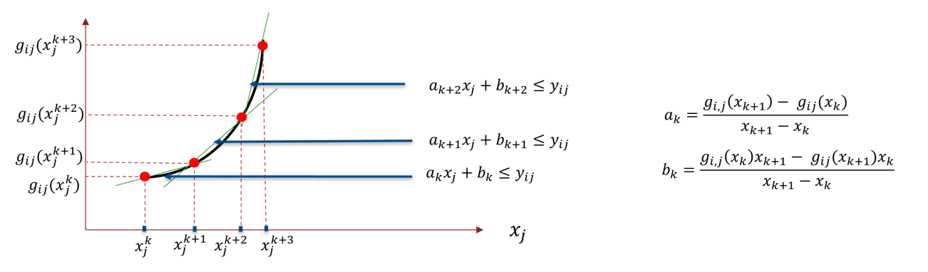
This reformulation obtains tighter approximations because, instead of adding just one cut at each iteration, you are adding numVars cuts per iteration. Furthermore, the univariate functions allow you to build a better initial approximation that helps to obtain an initial feasible point. The initial approximation is achieved with the inner cuts. Unlike the outer cuts that linearly approximate the nonlinear function with tangent lines, the inner cuts use secant lines.

Quadratic functions are not originally separable. By introducing two sets of auxiliary variables (y and t), you can rewrite all quadratic functions in a problem as separable functions as long as the matrix of the quadratic coefficients is positive semidefinite.

g(x)=xTQx+qTx+q00,g(x)=xT(STS)x+qTx+q00,      Q=STSg(x)=yTy+qTx+q00,                 y=Sx       g(x)=i=1n(ti+qixi)q0,                 yi2ti

Tips

You can also use dot notation to specify associated name-value options.

obj = obj.setSolverMINLP(Name,Value);

Note

The solverTypeMINLP and solverOptionsMINLP properties cannot be set using dot notation because they are hidden properties. To set the solverTypeMINLP and solverOptionsMINLP properties, use the setSolverMINLP function directly.

Algorithms

When any one, or any combination of 'Conditional' BoundType, MinNumAssets, or MaxNumAssets constraints is active, the portfolio problem is formulated by adding NumAssets binary variables. The binary variable 0 indicates that an asset is not invested and the binary variable 1 indicates that an asset is invested.

The MinNumAssets and MaxNumAssets constraints narrow down the number of active positions in a portfolio to the range of [minN, maxN]. In addition, the 'Conditional' BoundType constraint is to set a lower and upper bound so that the position is either 0 or lies in the range [minWgt, maxWgt]. These two types of constraints are incorporated into the portfolio optimization model by introducing n variables, νi, which only take binary values 0 and 1 to indicate whether the corresponding asset is invested (1) or not invested (0). Here n is the total number of assets and the constraints can be formulated as the following linear inequality constraints:

minNi=1nυi maxNminWgtυiximaxWgtυi0υ1υi are integers

In this equation, minN and maxN are representations for MinNumAsset and MaxNumAsset that are set using setMinMaxNumAssets. Also, minWgt and maxWgt are representations for LowerBound and UpperBound that are set using setBounds.

The portfolio optimization problem to minimize the variance of the portfolio, subject to achieving a target expected return and some additional linear constraints on the portfolio weights, is formulated as

minimizex  xTHxs.t.  mTxTargetReturnAxbAeqx=beqlbxub

In this equation, H represents the covariance and m represents the asset returns.

The portfolio optimization problem to maximize the return, subject to an upper limit on the variance of the portfolio return and some additional linear constraints on the portfolio weights, is formulated as

maximizex  mTxs.t.  xTHxTargetRiskAxbAeqx=beqlbxub

When the 'Conditional' BoundType, MinNumAssets, and MaxNumAssets constraints are added to the two optimization problems, the problems become:

minimizexυ  xTHxs.t.  mTxTargetReturnA'[x;υ]b'Aeqx=beqminNi=1nυimaxNminWgt(υi)ximaxWgt(υi)lbxub0υ1υi are integers

maximizexυ  mTxs.t.  xTHxTargetRiskA'[x;υ]b'Aeqx=beqminNi=1nυimaxNminWgtυiximaxWgt(υi)0υ1υi are integers

References

[1] Bonami, P., Kilinc, M., and J. Linderoth. "Algorithms and Software for Convex Mixed Integer Nonlinear Programs." Technical Report #1664. Computer Sciences Department, University of Wisconsin-Madison, 2009.

[2] Kelley, J. E. "The Cutting-Plane Method for Solving Convex Programs." Journal of the Society for Industrial and Applied Mathematics. Vol. 8, Number 4, 1960, pp. 703–712.

[3] Linderoth, J. and S. Wright. "Decomposition Algorithms for Stochastic Programming on a Computational Grid." Computational Optimization and Applications. Vol. 24, Issue 2–3, 2003, pp. 207–250.

[4] Nocedal, J., and S. Wright. Numerical Optimization. New York: Springer-Verlag, 1999.

Version History

Introduced in R2018b

expand all