Check Fit of Multiplicative ARIMA Model

R2026b

This example shows how to do goodness of fit checks. Residual diagnostic plots help verify model assumptions, and cross-validation prediction checks help assess predictive performance. The time series is monthly international airline passenger numbers from 1949 to 1960.

Load Data and Estimate Model

Load the airline data set.

load Data_Airline
y = log(Data);
T = length(y);

Mdl = arima(Constant=0,D=1,Seasonality=12,MALags=1,SMALags=12);
EstMdl = estimate(Mdl,y);

 
    ARIMA(0,1,1) Model Seasonally Integrated with Seasonal MA(12) (Gaussian Distribution):
 
                  Value      StandardError    TStatistic      PValue  
                _________    _____________    __________    __________

    Constant            0              0           NaN             NaN
    MA{1}        -0.37716       0.066794       -5.6466      1.6364e-08
    SMA{12}      -0.57238       0.085439       -6.6992      2.0952e-11
    Variance    0.0012634     0.00012395        10.193      2.1406e-24

Check Residuals for Normality

One assumption of the fitted model is that the innovations follow a Gaussian distribution. Infer the residuals, and check them for normality.

res = infer(EstMdl,y);
stres = res/sqrt(EstMdl.Variance);
x = -4:.05:4;
[f,xi] = ksdensity(stres);

figure
tiledlayout(1,2);
nexttile;
qqplot(stres)

nexttile;
plot(xi,f,LineWidth=2)
hold on
plot(x,normpdf(x),LineWidth=2)
legend("Standardized Residuals","Standard Normal")
hold off

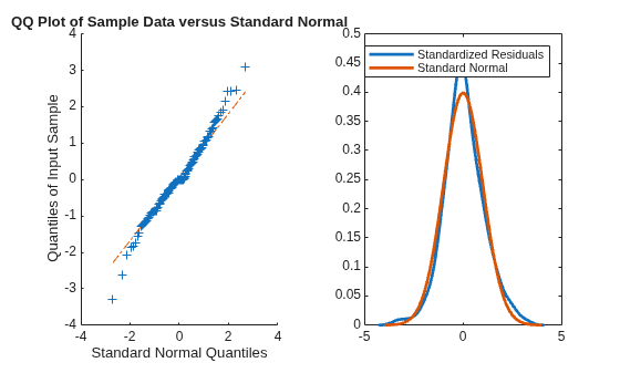
The quantile-quantile plot (QQ-plot) and kernel density estimate show no obvious violations of the normality assumption.

Check Residuals for Autocorrelation

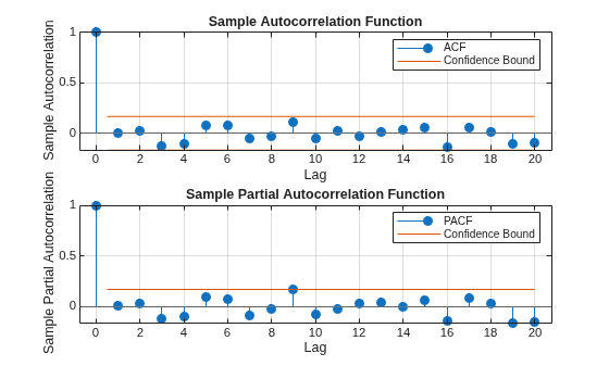
Confirm that the residuals are uncorrelated. Look at the sample autocorrelation function (ACF) and partial autocorrelation function (PACF) plots for the standardized residuals.

figure
subplot(2,1,1)
autocorr(stres)
subplot(2,1,2)
parcorr(stres)

[h,p] = lbqtest(stres,Lags=[5,10,15],DoF=[3,8,13])

h = 1×3 logical array

   0   0   0

p = 1×3

    0.1842    0.3835    0.7321

The sample ACF and PACF plots show no significant autocorrelation. More formally, conduct a Ljung-Box Q-test at lags 5, 10, and 15, with degrees of freedom 3, 8, and 13, respectively. The degrees of freedom account for the two estimated moving average coefficients.

The Ljung-Box Q-test confirms the sample ACF and PACF results. The null hypothesis that all autocorrelations are jointly equal to zero up to the tested lag is not rejected (h = 0) for any of the three lags.

Check Predictive Performance

Use a holdout sample to compute the predictive MSE of the model. Use the first 100 observations to estimate the model, and then forecast the next 44 periods.

y1 = y(1:100);
y2 = y(101:end);

Mdl1 = estimate(Mdl,y1);

 
    ARIMA(0,1,1) Model Seasonally Integrated with Seasonal MA(12) (Gaussian Distribution):
 
                  Value      StandardError    TStatistic      PValue  
                _________    _____________    __________    __________

    Constant            0              0           NaN             NaN
    MA{1}        -0.35674       0.089461       -3.9876      6.6739e-05
    SMA{12}      -0.63319       0.098744       -6.4124      1.4326e-10
    Variance    0.0013285     0.00015882         8.365       6.013e-17

yF1 = forecast(Mdl1,44,Y0=y1);
pmse = mean((y2-yF1).^2)

pmse = 
0.0069

figure
plot(y2,LineWidth=2)
hold on
plot(yF1,LineWidth=1.5)
xlim([0,44])
title("Prediction Error")
legend("Observed","Forecast",Location="northwest")
hold off

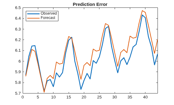
The predictive ability of the model is quite good. You can optionally compare the PMSE for this model with the PMSE for a competing model to help with model selection.