lbqtest
Ljung-Box Q-test for residual autocorrelation
Syntax
Description
h = lbqtest(res)
StatTbl = lbqtest(Tbl)DataVariable name-value argument.
[___] = lbqtest(___,
specifies options using one or more name-value arguments in
addition to any of the input argument combinations in previous syntaxes.
Name=Value)lbqtest returns the output argument combination for the
corresponding input arguments.
Some options control the number of tests to conduct. The following conditions
apply when lbqtest conducts multiple tests:
For example,
lbqtest(Tbl,DataVariable="ResidualGDP",Alpha=0.025,Lags=[1
                    4])
conducts two tests, at a level of significance of 0.025, for the
presence of residual autocorrelation in the variable ResidualGDP
of the table Tbl. The first test includes 1
lag in the test statistic, and the second test includes 4
lags.
Examples
Test a time series for residual autocorrelation using default options of lbqtest. Input the time series data as a numeric vector.
Load the Deutschmark/British pound foreign-exchange rate data set.
load Data_MarkPoundData is a time series vector of daily Deutschmark/British pound bilateral spot exchange rates.
Plot the series.
plot(Data)
title("\bf Deutschmark/British Pound Bilateral Spot Exchange Rate")
ylabel("Spot Exchange Rate")
xlabel("Business Days Since January 2, 1984")
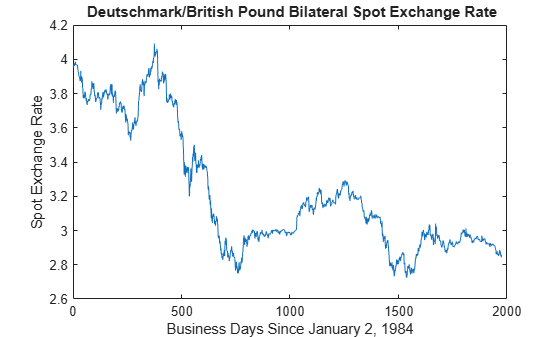
The series appears nonstationary.
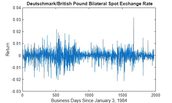
To stabilize the series, convert the spot exchange rates to returns.
returns = price2ret(Data);

plot(returns)
title("\bf Deutschmark/British Pound Bilateral Spot Exchange Rate")
ylabel("Return")
xlabel("Business Days Since January 3, 1984")
Compute the deviations of the return series from the mean.
residuals = returns - mean(returns);
At 0.05 level of significance, test the residual series for autocorrelation using the default options of the Ljung-Box Q-test.
h = lbqtest(residuals)
h = logical
   0
The result h = 0 indicates that insufficient evidence exists to reject the null hypothesis of no residual autocorrelation through 20 lags.
Load the Deutschmark/British pound foreign-exchange rate data set.
load Data_MarkPoundPreprocess the data by following this procedure:
Stabilize the series by computing daily returns.
Compute the deviations from the mean return.
returns = price2ret(Data);
residuals = returns - mean(returns);
Test the residual series for a significant autocorrelation from 1 through 20 lags. Return the test decision, -value, test statistic, and critical value.
[h,pValue,stat,cValue] = lbqtest(residuals)
h = logical
   0
pValue =
0.1131
stat =
27.8445
cValue =
31.4104
Test a time series, which is one variable in a table, for residual autocorrelation using default options of lbqtest.
Load the equity index data set Data_EquityIdx. Preprocess the daily NASDAQ closing prices by performing the following actions:
Convert the price series to a percentage return series by using
price2ret.Represent the series as residuals that fluctuate around a constant level by centering the returns series.
Store the residual series in the table with the rest of the data. Because the price-to-return conversion reduces the sample size from the head of the series, replace the missing residual with the a NaN.
load Data_EquityIdx
ret = 100*price2ret(DataTable.NASDAQ);
res = ret - mean(ret);
DataTable.Residuals_NASDAQ = [NaN; res];
DataTable.Properties.VariableNames{end}
ans = 'Residuals_NASDAQ'
The residual series is the last variable in the table.
Conduct Ljung-Box Q-test on the residual series at a 5% significance level by supplying the entire data set lbqtest.
StatTbl = lbqtest(DataTable)
StatTbl=1×7 table
                h        pValue       stat     cValue    Lags    Alpha    DoF
              _____    __________    ______    ______    ____    _____    ___

    Test 1    true     2.8182e-11    92.395    31.41      20     0.05     20
lbqtest returns test results and settings in the table StatTbl, where variables correspond to test results (h, pValue, stat, and cValue) and settings (Lags, Alpha, and DoF), and rows correspond to individual tests (in this case, lbqtest conducts one test).
h = 1 and pValue = 2.82e-11 rejects the null hypothesis and suggests that the evidence for at least one significant autocorrelation in lags 1 through 20 in the NASDAQ returns residual series is strong.
By default, lbqtest tests the last variable in the table. To select a variable from an input table to test, set the DataVariable option.
Load the Deutschmark/British pound foreign-exchange rate data set.
load Data_MarkPoundConvert the prices to returns.
returns = price2ret(Data);
Compute the deviations of the return series.
res = returns - mean(returns);
Test the hypothesis that the residual series is not autocorrelated, using the default number of lags.
h1 = lbqtest(res)
h1 = logical
   0
h1 = 0 indicates that there is insufficient evidence to reject the null hypothesis that the residuals of the returns are not autocorrelated.
Test the hypothesis that there are significant ARCH effects, using the default number of lags [3].
h2 = lbqtest(res.^2)
h2 = logical
   1
h2 = 1 indicates that there are significant ARCH effects in the residuals of the returns.
Test for residual heteroscedasticity using archtest. Specify an alternative ARCH() model, where , for consistency with h2.
h3 = archtest(res,Lags=20)
h3 = logical
   1
h3 = 1 indicates that the null hypothesis of no residual heteroscedasticity should be rejected in favor of an ARCH() model, where . This result is consistent with h2.
Conduct multiple Ljung-Box Q-tests for autocorrelation by specifying several lags for the test statistic. The data set is a time series of 57 consecutive days of overshorts from an underground gasoline tank in Colorado [2]. That is, the current overshort () represents the accuracy in measuring the amount of fuel:
In the tank at the end of day
In the tank at the end of day
Delivered to the tank on day
Sold on day .
Load the data set.
load Data_Overshort
T = height(DataTable);

figure
plot(DataTable.OSHORT)
title('Daily Gasoline Overshorts')
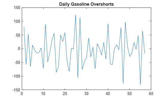
lbqtest is appropriate for a series with a constant mean. Because the series appears to fluctuate around a constant mean, you do not need to stabilize it.
Compute deviations from the mean.
DataTable.Residuals_OSHORT = DataTable.OSHORT - mean(DataTable.OSHORT);
Assess whether the residuals are autocorrelated. Include 5, 10, and 15 lags in the test statistic, and adjust the significance level of each test to 0.05/3.
StatTbl = lbqtest(DataTable,DataVariable="Residuals_OSHORT", ...
    Lags=[5 10 15],Alpha=0.05/3)
StatTbl=3×7 table
                h        pValue       stat     cValue    Lags     Alpha      DoF
              _____    __________    ______    ______    ____    ________    ___

    Test 1    true      0.0016465     19.36    13.839      5     0.016667     5
    Test 2    true     0.00068328    30.599    21.707     10     0.016667    10
    Test 3    true       0.001281    36.964     28.88     15     0.016667    15
Rows of StatTbl contain results of separate tests conducted for each specified lag. Each test rejects the null hypothesis at 0.0167 level of significance.
Infer residuals from an estimated ARIMA model, and assess whether the residuals exhibit autocorrelation using lbqtest.
Load the Australian Consumer Price Index (CPI) data set. The time series (cpi) is the log quarterly CPI from 1972 to 1991. Remove the trend in the series by taking the first difference.
load Data_JAustralian
cpi = DataTable.PAU;
T = length(cpi);
dCPI = diff(cpi);
dt = datetime(dates,ConvertFrom="datenum");

figure
plot(dt(2:T),dCPI)
title("Differenced Australian CPI")
xlabel("Year")
ylabel("CPI Growth Rate")
axis tight
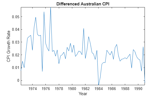
The differenced series appears stationary.
Fit an AR(1) model to the series, and then infer residuals from the estimated model.
Mdl = arima(1,0,0);
EstMdl = estimate(Mdl,dCPI);
    ARIMA(1,0,0) Model (Gaussian Distribution):

                  Value      StandardError    TStatistic      PValue
                _________    _____________    __________    __________

    Constant     0.015564      0.0028766        5.4106      6.2808e-08
    AR{1}         0.29646        0.11048        2.6834       0.0072876
    Variance    0.0001038     1.1932e-05        8.6994      3.3362e-18
res = infer(EstMdl,dCPI);
stdRes = res/sqrt(EstMdl.Variance); % Standardized residuals
Assess whether the residuals are autocorrelated by conducting a Ljung-Box Q-test. The standardized residuals originate from the estimated model (EstMdl) containing parameters. When using such residuals, perform the following actions:
Adjust the degrees of freedom (
DoF) of the test statistic distribution to account for the estimated parameters.Set the number of lags to include in the test statistic.
When you count the estimated parameters, skip the constant and variance parameters.
lags = 10;
dof  = lags - 1; % One autoregressive parameter

[h,pValue] = lbqtest(stdRes,Lags=lags,DoF=dof)
h = logical
1
pValue =
0.0119
pValue = 0.0119 suggests that the residuals have significant autocorrelation in at least one lag of lags 1 through 5, at the 5% level.
Input Arguments
Name-Value Arguments
Output Arguments
More About
Tips
If you obtain the input residual series by fitting a model to data, reduce the degrees of
freedom DoF by the number of estimated coefficients, excluding
constants. For example, if you obtain the input residuals by fitting an
ARMA(p,q) model, set
DoF=L−p−q,
where L is the value of Lags.
Algorithms
The value of the
Lagsargument L affects the power of the test.If L is too small, the test does not detect high-order autocorrelations.
If L is too large, the test loses power when a significant correlation at one lag is washed out by insignificant correlations at other lags.
Box, Jenkins, and Reinsel suggest the default setting
Lags=min[20,T-1][1].Tsay cites simulation evidence showing better test power performance when L is approximately
log(T)[5].
lbqtestdoes not directly test for serial dependencies other than autocorrelation. However, you can use it to identify conditional heteroscedasticity (ARCH effects) by testing squared residuals [4].Engle's test assesses the significance of ARCH effects directly. For details, see
archtest.
References
[1] Box, George E. P., Gwilym M. Jenkins, and Gregory C. Reinsel. Time Series Analysis: Forecasting and Control. 3rd ed. Englewood Cliffs, NJ: Prentice Hall, 1994.
[2] Brockwell, P. J. and R. A. Davis. Introduction to Time Series and Forecasting. 2nd ed. New York, NY: Springer, 2002.
[3] Gourieroux, C. ARCH Models and Financial Applications. New York: Springer-Verlag, 1997.
[4] McLeod, A. I. and W. K. Li. "Diagnostic Checking ARMA Time Series Models Using Squared-Residual Autocorrelations." Journal of Time Series Analysis. Vol. 4, 1983, pp. 269–273.
[5] Tsay, R. S. Analysis of Financial Time Series. 2nd Ed. Hoboken, NJ: John Wiley & Sons, Inc., 2005.
Version History
Introduced before R2006a