Generate RoadRunner Scene Using Aerial Lidar Data

This example uses:

This example shows how to generate a scene containing roads and static objects by using aerial lidar and OpenStreetMap data. In this example, you extract trees, buildings, and road elevation information from lidar data, and reconstruct a road network by using the OpenStreetMap data.

You can create a virtual scene from recorded sensor data that represents real-world scenes and use it to perform verification and validation of automated driving functionalities. Lidar point clouds enable you to accurately extract the locations and dimensions of static objects in a scene, while OpenStreetMap provides access to worldwide, crowd-sourced map data. Using both the lidar data and the OpenStreetMap road network data, you can create a scene in RoadRunner that contains roads and other objects, such as trees and buildings.

In this example, you:

Load and visualize the USGS aerial point cloud data.
Perform semantic segmentation by using a pretrained deep learning network.
Unproject the point cloud to local coordinates, and create a georeferenced point cloud.
Extract trees and buildings from the lidar point cloud.
Extract roads from the OpenStreetMap and lidar data.
Build and view the RoadRunner scene.

Load Lidar Data

This example requires the Scenario Builder for Automated Driving Toolbox™ support package. Check if the support package is installed and, if not, install it using the Add-On Manager. For more information on installing support packages, see Get and Manage Add-Ons.

checkIfScenarioBuilderIsInstalled

This example uses aerial point cloud data downloaded from the U.S. Geological Survey (USGS) 3DEP LidarExplorer [1]. This is an online platform that provides access to recorded lidar data in LAZ format for various regions of the United States. To download lidar data, in the 3DEP LidarExplorer, hold Ctrl and drag to draw a rectangular area of interest on the map. The USGS Lidar Explorer shows a list of available lidar data in the selected region. Select a data set from the list, and download the lidar point cloud as a LAZ file.

For this example, download a ZIP file containing lidar data from the 3DEP LidarExplorer, and then unzip the file. Load the point cloud data into the workspace using the readPointCloud (Lidar Toolbox) function of the lasFileReader (Lidar Toolbox) object, and visualize the point cloud.

dataFolder = tempdir;
lidarDataFileName = "USGSLidarExplorerData.zip"; 
url = "https://ssd.mathworks.com/supportfiles/driving/data/" + lidarDataFileName; 
filePath = fullfile(dataFolder,lidarDataFileName); 
if ~isfile(filePath)
    websave(filePath,url)
end
unzip(filePath,dataFolder)

% Specify the path of the downloaded LAZ file.
lasfile = fullfile(dataFolder,"USGS_LPC_CA_NoCAL_3DEP_Supp_Funding_2018_D18_w2276n1958.laz");

% Create a lasFileReader object.
lasReader = lasFileReader(lasfile);

% Read the point cloud.
registeredPointCloud = readPointCloud(lasReader);

Visualize the central region of the point cloud using the helperViewPointCloudCenterRegion helper function. To visualize the complete point cloud, you can use the pcshow function.

helperViewPointCloudCenterRegion(registeredPointCloud)
title("USGS Aerial Lidar Data: Central region")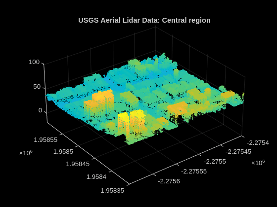

Segment Point Clouds Using Deep Learning

In this example, you use a pretrained RandLANet semantic segmentation network to segment the trees and buildings in the point cloud data.

The input point cloud in this example covers an area of 1000-by-1000 meters, which is much larger than the typical area covered by terrestrial rotating lidars. For efficient memory processing, divide the point cloud into small, non-overlapping blocks of size 200-by-200 meters, and then perform the semantic segmentation on each block of the blocked point cloud by using the helperRandLANetSegmentObjects helper function.

% Segment the non-ground point cloud to perform segmentation.
[~,pc,~] = segmentGroundSMRF(registeredPointCloud);

% Load the color map.
cmap = helperAerialLidarColorMap;

% Set the size of the blocks for the blocked point cloud.
bpdSizeinMeters = [200 200];

% Perform segmentation using the helperRandLANetSegmentObjects function, and store the results in labels.
labels = helperRandLANetSegmentObjects(pc,bpdSizeinMeters);

To help visualize the results, map the labels of all the points of the point cloud to the Color property of the point cloud registeredPointCloud using the colormap as defined by the helperAerialLidarColorMap helper function. Visualize the labels of the central region of the point cloud by using the helperViewPointCloudCenterRegion helper function.

pc.Color = cell2mat(cmap(labels));
helperViewPointCloudCenterRegion(pc)
title("USGS Aerial Lidar Data: Central region")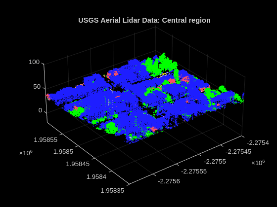

Unproject Point Cloud to Local Coordinates and Create Georeferenced Point Cloud

The point cloud loaded from the LAZ file is in a projected coordinate system. By converting the point cloud data from a projected coordinate system to a local coordinate system, you can ensure accurate spatial analysis, and measurements tailored to the specific region of interest. This transformation ensures that the point cloud matches with the road network from OpenStreetMap.

Read the coordinate reference system data from the LAZ file by using the readCRS (Lidar Toolbox) function.

crs = readCRS(lasReader);

% Extract the locations and intensity from the segmented point cloud.
x = pc.Location(:,1);
y = pc.Location(:,2);
z = pc.Location(:,3);
pcintensity = pc.Intensity;

% Extract the color, which contains the segmentation labels obtained in the previous section.
pccolor = pc.Color;

Then, unproject the xy-coordinates of the map to latitude-longitude coordinates by using the projinv (Mapping Toolbox) function. Select the mean values of the latitude, longitude, and altitude to define the georeference for the point cloud.

Note: You must use the same georeference to download the road network of interest from OpenStreetMap.

[lat,lon] = projinv(crs,x,y);
geoReference = [mean(lat) mean(lon) mean(z)];

Convert the latitude, longitude, and altitude to the local coordinate system with the georeference as the origin, and create a georeferenced point cloud.

[xE,yN,zU] = latlon2local(lat,lon,z,geoReference);
pc = pointCloud([xE yN zU],Color=pccolor,Intensity=pcintensity);

Extract Trees and Buildings from Georeferenced Point Cloud

To generate a RoadRunner Scene containing static objects such as trees and buildings, you must have a cuboid parameters array containing the center, dimension, and orientation for each static object.

First, specify the labels for which to extract cuboid parameters.

labelNames = ["vegetation","buildings"];

Create a parameters structure that contains a field for each specified label. Specify each label field as a structure containing the fields minDistance and NumClusterPoints, where minDistance specifies the minimum distance between points of two different static objects, and NumClusterPoints specifies either the minimum or the minimum and maximum number of points to include in each static object, based on the density of point cloud.

If static objects of the same type are very close to each other, reduce the minDistance value to identify them.

vegetationParams = struct("minDistance",1.3,"NumClusterPoints",[250 1500]);
buildingParams = struct("minDistance",0.8,"NumClusterPoints",500);

parameters = struct("vegetation",vegetationParams,"buildings",buildingParams);

Use the helperExtractCuboidsFromLidar helper function, attached to this example as a supporting file, to obtain the cuboid parameters for each instance of a static object with the specified labels from the point cloud, and store the parameters in a cell array cuboids.

Based on the size and resolution of the point cloud, this section may take more time to run. To tune the minDistance and NumClusterPoints parameters on a smaller point cloud of size 150-by-150 meters, set doTuning to true. After getting satisfactory results, set doTuning to false to obtain cuboid parameters for the complete point cloud.

doTuning = false;

if doTuning
    % Extract points inside ROI of 150-by-150 meter center region of the point cloud.
    roiSmall = [-150 150 -150 150 pc.ZLimits];
    idx = findPointsInROI(pc,roiSmall);
    pcROI = select(pc,idx);
    % Extract the cuboid parameters.
    cuboids = helperExtractCuboidsFromLidar(pcROI,parameters,labelNames,cmap);
    ax = pcshow(pcROI,ViewPlane="XY");
else
    % Extract the cuboid parameters for the complete region of the point cloud.
    cuboids = helperExtractCuboidsFromLidar(pc,parameters,labelNames,cmap);
    ax = pcshow(pc,ViewPlane="XY");
end

Visualize the cuboid parameters overlaid on the point cloud.

hold on
% Overlay the vegetation cuboids in red color and buildings in cyan color.
showShape("cuboid",cuboids{1},Color="red",Parent=ax)
showShape("cuboid",cuboids{2},Color="cyan",Parent=ax)
hold off

Note: Because of the low resolution of the point clouds, several buildings are closer to their neighboring buildings than in reality. Some of the extracted buildings might be oriented incorrectly, or overlap with other buildings.

The lidar data used in this example has been recorded by an aerial lidar sensor with a bird's-eye field of view, so the majority of the points in the point cloud are on the tops of buildings and trees, with very few points on the sides. As a result, the cuboids extracted from point cloud might not be accurate, and a scene generated with this data might place some objects in the air. To extend the height of the objects to the ground plane, using information from the point cloud, use the helperExtendCuboidsToGround function, attached to this example as a supporting file.

for i = 1:height(cuboids)
    cuboids{i} = helperExtendCuboidsToGround(cuboids{i},pc);
end

The area contains buildings of different heights. To generate RoadRunner asset paths for buildings based on their heights, use the helperGenerateAssetPaths helper function, attached to this example as a supporting file.

statObjs.trees = cuboids{1};
statObjs.buildings = cuboids{2};

% Generate RoadRunner asset paths for buildings.
[statObjs.buildings, params.buildings.AssetPath] = helperGenerateAssetPaths("buildings",statObjs.buildings);

Generate static object information in the RoadRunner HD Map format by using the roadrunnerStaticObjectInfo function.

objectsInfo = roadrunnerStaticObjectInfo(statObjs,Params=params);

Extract Roads using OpenStreetMap and Lidar

To add the road network into the RoadRunner Scene, first download the map file from the OpenStreetMap (OSM) [2] website for the same area that represents the downloaded lidar data.

Import the OSM road network by using the getMapROI function. Use the georeference of the point cloud as the latitude and longitude value for the OSM road network, and the mean of the limits of the point cloud pc as the extent of the road network. To get the road network in the RoadRunner HD Map format, import the roads from the OpenStreetMap web service into a driving scenario and use the getRoadRunnerHDMap function.

osmExtent = mean(abs([pc.XLimits pc.YLimits]));
mapParameters = getMapROI(geoReference(1),geoReference(2),Extent=osmExtent);
osmFileName = websave("RoadScene.osm",mapParameters.osmUrl,weboptions(ContentType="xml"));
scenario = drivingScenario;
roadNetwork(scenario,"OpenStreetMap",osmFileName)

% Get the roadrunnerHDMap object from the drivingScenario object.
rrMap = getRoadRunnerHDMap(scenario);

As the elevation information for the road might not be accurate, improve the road elevation with reference to the point cloud by using helperRoadRunnerElevateLane helper function, attached to this example as a supporting file.

laneInfo = helperRoadRunnerElevateLane(rrMap,pc);

Create and Build RoadRunner Scene

Use the laneInfo and objectsInfo obtained in the previous sections to create a RoadRunner Scene containing roads and static objects respectively.

Update the RoadRunner HD Map using the road network with improved elevation data.

rrMap.Lanes = laneInfo.Lanes;
rrMap.LaneBoundaries = laneInfo.LaneBoundaries;
rrMap.LaneGroups = laneInfo.LaneGroups;

Update the map with the information on the trees and buildings..

rrMap.StaticObjectTypes = objectsInfo.staticObjectTypes;
rrMap.StaticObjects = objectsInfo.staticObjects;

Plot the map, which contains information for the static objects, lane boundaries, and lane centers.

f = figure(Position=[1000 818 700 500]);
ax = axes("Parent",f);
plot(rrMap,ShowStaticObjects=true,Parent=ax)

Write the RoadRunner HD Map to a binary file, which you can import into the Scene Builder Tool.

rrMapFileName = "RoadRunnerAerialScene.rrhd";
write(rrMap,rrMapFileName)

Open the RoadRunner application by using the roadrunner (RoadRunner) object. Import the RoadRunner HD Map data from your binary file, and build it in the currently open scene.

Specify the path to your local RoadRunner installation folder. This code shows the path for the default installation location on Windows®.

rrAppPath = "C:\Program Files\RoadRunner " + matlabRelease.Release + "\bin\win64";

Specify the path to your RoadRunner project. This code shows the path to a sample project folder on Windows.

rrProjectPath = "C:\RR\MyProject";

Open RoadRunner using the specified path to your project

rrApp = roadrunner(rrProjectPath,InstallationFolder=rrAppPath);

Copy the RoadRunnerAerialScene.rrhd scene file into the Asset folder of the RoadRunner project, and import it into RoadRunner.

copyfile(rrMapFileName,(rrProjectPath + filesep + "Assets"));
rrhdFile = fullfile(rrProjectPath,"Assets",rrMapFileName);

Clear the overlap groups option to enable RoadRunner to create automatic junctions at the geometric overlap of the roads.

enableOverlapGroupsOpts = enableOverlapGroupsOptions(IsEnabled=0);
buildOpts = roadrunnerHDMapBuildOptions(EnableOverlapGroupsOptions=enableOverlapGroupsOpts);
importOptions = roadrunnerHDMapImportOptions(BuildOptions=buildOpts);

Import the scene into RoadRunner by using the importScene function.

importScene(rrApp,rrhdFile,"RoadRunner HD Map",importOptions)

Note: Use of the Scene Builder Tool requires a RoadRunner Scene Builder license, and use of RoadRunner Assets requires a RoadRunner Asset Library Add-On license.

This figure shows an aerial point cloud and the corresponding RoadRunner Scene built using RoadRunner Scene Builder.

USGS RoadRunner Scene

Helper Functions

helperRandLANetSegmentObjects — A helper function to perform semantic segmentation on a point cloud.

function labels = helperRandLANetSegmentObjects(ptCld,blockSize)
    % A helper function to perform semantic segmentation on point cloud.
    % Initialize the RandlaNet segmentor trained on Dales data.
    segmentor = randlanet("dales");
    
    % Initialize prediction labels.
    labels = strings([ptCld.Count 1]);
    
    % Calculate the number of non-overlapping grids based on gridSize, XLimits,
    % and YLimits of the point cloud.
    numGridsX = round(diff(ptCld.XLimits)/blockSize(1));
    numGridsY = round(diff(ptCld.YLimits)/blockSize(2));
    [~,~,~,indx,indy] = histcounts2(ptCld.Location(:,1),ptCld.Location(:,2), ...
    [numGridsX numGridsY],XBinLimits=ptCld.XLimits,YBinLimits=ptCld.YLimits);
    ind = sub2ind([numGridsX numGridsY],indx,indy);
    
    % Read each grid and predict labels on each grid.    
    for num = 1:numGridsX*numGridsY
        idx = ind==num;
        ptCloudDense = select(ptCld,idx);
        predLabels = segmentObjects(segmentor,ptCloudDense);
        labels(idx) = predLabels;
    end
end

helperAerialLidarColorMap — Color map for the lidar labels.

function cmap = helperAerialLidarColorMap
    % This function contains the color map for the lidar labels.
    labelNames = ["ground", ...
        "vegetation", ...
        "cars", ...
        "trucks", ...
        "powerlines", ...
        "fences", ...
        "poles", ...
        "buildings"];

    labelColors = {uint8([255 150 255]), ...
        uint8([0 255 0 ]), ...
        uint8([245 150 100]), ...
        uint8([250 80 100]), ...
        uint8([255 255 0 ]), ...
        uint8([204 204 255]), ...
        uint8([192 192 192]), ...
        uint8([30 30 255])};

    cmap = dictionary(labelNames,labelColors);
end

helperViewPointCloudCenterRegion — Visualizes the central region of a registered point cloud.

function helperViewPointCloudCenterRegion(ptCld)
    
    % Define the ROI
    cent = [sum(ptCld.XLimits)/2,sum(ptCld.YLimits)/2];
    roi = [cent(1)-150 cent(1)+100 cent(2)-150 cent(2)+100 ptCld.ZLimits];
    pcViz = select(ptCld,findPointsInROI(ptCld,roi));
    % Visualize the point cloud.
    pcshow(pcViz)
end

References

[1] 3DEP LidarExplorer courtesy of the U.S. Geological Survey https://apps.nationalmap.gov/lidar-explorer/.

[2] You can download OpenStreetMap files from https://www.openstreetmap.org, which provides access to crowd-sourced map data all over the world. The data is licensed under the Open Data Commons Open Database License (ODbL), https://opendatacommons.org/licenses/odbl/.