Modeling 5G Non-Terrestrial Network (NTN) Links in MATLAB - MATLAB
Video Player is loading.
Current Time 0:00
Duration 40:21
Loaded: 0.41%
Stream Type LIVE
Remaining Time 40:21
 
1x
  • Chapters
  • descriptions off, selected
  • en (Main), selected
    Video length is 40:21

    Modeling 5G Non-Terrestrial Network (NTN) Links in MATLAB

    Overview

    Ubiquitous internet connectivity using satellites is no longer a dream as demonstrated by the 3GPP investment in 5G New Radio (NR) non-terrestrial networks (NTN). The challenges of NTN links are very different in comparison to terrestrial links, as they must deal with larger propagation delays and high Doppler.

    In this webinar, you will learn about modeling 5G non-terrestrial links in MATLAB. We will start with an overview of the orbit propagation capabilities in MATLAB that allows you to model large satellites constellations in their orbits and generate coverage maps for different antenna types. We will then focus modeling a 5G NTN link by evaluating the throughput of NR Physical Downlink Shared Channel (PDSCH) in an NTN channel, specifically, the tapped delay line (TDL) NTN channel. We will also learn about the different Doppler compensation strategies employed in an NTN link. We will also briefly talk about narrowband Internet of Things (NB-IoT) NTN links before making our conclusions. 

    Highlights

    Highlights include:

    • Modeling large satellite constellations
    • Satellite link budgets
    • Generating coverage maps on earth for different antenna types
    • 5G NR NTN PDSCH throughput in the presence of RF Impairments
    • NB-IoT throughput for an NTN link

    About the Presenter

    Mike McLernon is an advocate for communications and software-defined radio products at MathWorks. Since joining MathWorks in 2001, he has overseen the development of PHY layer modeling and SDR connectivity capabilities in Communications Toolbox. He has worked in the communications field for over 30 years in both the satellite and wireless industries. Mike received his BSEE from the University of Virginia and his MEEE from Rensselaer Polytechnic Institute.

    Recorded: 29 Jan 2025

    Hello, and welcome to Modeling 5G Non-Terrestrial Networks in MATLAB. My name is Mike McLernon. I've been with MathWorks since 2001, many of those years in the development organization, building all kinds of wireless capabilities, channel models, reference receiver designs, RF modeling, software-defined radio connectivity. More recently, I have been in the technical marketing group.

    I have been integrally involved with the satellite communications toolbox, which we'll be talking about today, for roughly five or six years. So NTNs is a topic that is very, very relevant and hot right now. So let's just dive in.

    Here's what we'll be talking about today. We'll first motivate the topic, talk about use cases, challenges, architectures, et cetera. So let's begin.

    First of all, let's define, what is NTN or non-terrestrial network? First, you start with a terrestrial network, a TN. You see an urban area with some base stations. Now, you add satellites to the mix. Some of them may be in Low Earth Orbit, or LEO, some in Medium Earth Orbit, or MEO, some in Geosynchronous Orbit or GEO.

    Then you have some downlinks. And so you may use these NTSs for backhaul to connect directly to the 5G core network. You can also use it to connect to remote assets like ships in the open ocean.

    You can utilize space-to-air and air-to-space links with NTSs, service links with both UEs and VSATs, which have very, very different power budget architectures, which we will talk about in a little bit, HAPS, or High-Altitude Platform Systems, often balloons that might float at 10 to 20 kilometers above the surface. Also, if you are talking about LEO orbits, which most folks are these days, you have to consider inter-satellite links.

    So that is basically the architecture of what an NTN could look like in the very, very near future. Let's ask, why NTSs? So you see in this spinning globe, there is a whole lot of the globe that is unpopulated. It may be true that roughly 80% of the world's population is covered by the terrestrial network right now. But 80% of the landmass is not.

    And so NTSs want to address these unconnected areas right now, first, remote areas, as we see, ships on the open ocean; rural areas where it's just economically infeasible to put down a terrestrial network; disaster recovery-- we may recall that a few years ago during some Florida hurricanes, the cellular infrastructure was knocked out. Satellites came to the rescue to connect first responders, medical personnel, et cetera-- also, surprisingly, in urban environments, where if the terrestrial network is just overloaded, satellites can come in and offload some of that bandwidth.

    Let's also build out our diagram here and talk about ubiquitous connectivity. We start with a personal area network, where it operates on a scale of meters-- Bluetooth is a prime example-- local area networks, which operate on the scale of tens to maybe a few hundred meters-- WiFi is the shining example there-- a wide area network, which may cover a city, a metropolitan area, cellular 5G, LTE. Those are the poster children applications there.

    And finally, for a global area network, satellites are involved. And we are seeing now that 5G also is involved in the global area network. And it will only become more so when 6G gets fielded in roughly 2029, 2030.

    Let's talk a little bit about the NTN timeline. So even though NTN are just now in 2024 beginning to be deployed, people in 3GPP, the standards body for cellular, they were thinking about it in 2018. They defined very high-level deployment scenarios and channel models.

    And you can see, in each release afterwards, every year or two later, more specificity has been built into the standards up until most recently with R18 being released, we're talking about RF and coexistence requirement, L-- and S-band operation. So this spec is getting more and more solidified as time goes on.

    Let's talk a little bit more about use cases. Here's our diagram that we showed a moment ago. Let's drill into some of the unique scenarios where use cases apply. In an urban area, again, we talked about traffic offload-- network resilience. So NTNs are meant primarily to provide network ubiquity and resilience and reliability. And so that's where it will really happen in an urban environment.

    In a rural environment, you would use NTNs for emergency service and wide area connectivity because there are vast areas of rural area where there is little to no terrestrial infrastructure. In remote areas, you would want public protection and disaster relief, as we spoke a moment ago. And for these isolated areas, which are aeronautical, Maritime, you want to build a remote hotspot. So NTNs are used in all of these applications.

    Let's talk about some of the technology challenges that are presented with NTNs. First off, beamforming an array design-- now, beamforming, certainly in the terrestrial world, is nothing new. People have been doing it for quite some time. But it is relatively new in the satellite world.

    And we are not talking about little 4x4 arrays. We have spoken to individuals that are interested in building arrays with 1,000 different elements. That presents significant RF phase coherence challenges.

    Also, with inter-satellite links, there are problems with or there can be problems with interference. There are architecture trade offs to figure out. Do you want to go with an RF link or an optical link? We'll talk about that in a little bit. Also, the routing and the scheduling and the networking is a big challenge when you have literally thousands of assets orbiting the Earth. And also, the physical layer also affects your routing and your scheduling, so very, very, very challenging.

    In addition, there's satellite maintenance, control, and housekeeping. If you are launching birds up in the air, you cannot send a repair man up there in case something breaks. You can mitigate that just with redundancy. And so but that means more higher launch costs. There are different UE designs. We alluded to this a little bit ago.

    UEs-- handsets, smartphones-- they would have very poor G over Ts. VSATs, on the other hand, which often use larger antennas, maybe even phased arrays, they would have a better G on T. So it really impacts different link budgets and RF design.

    Long, round trip times-- so the RTT, Round Trip Time, it is significantly longer for satellite links than for terrestrial links. And that really changes the protocol, the networking and the HARQ protocol. So we'll talk about that a little bit more later.

    There's carrier frequency offset. If you are using LEOs, which really zip around the Earth very, very quickly, you will get significant dopplers on the order of several hundred kilohertz. That really implicates challenges in your receiver design to be able to synchronize absolutely in frequency and phase for the received waveforms.

    Path loss-- so now you see, for a terrestrial link at a certain frequency, 2 gigahertz, your loss may be what? 112 db. But for an NTN Leo at 1,000 kilometers up, your path loss is going to be almost 50 dB greater. So that implicates RF design and antenna design greatly.

    Also, polarization mismatch-- as waves travel through the ionosphere, you are going to get Faraday rotation, which is going to create some mismatch and some loss. These have to be accounted for in a link budget calculation.

    Let's talk about some of these architectures. OK, this is a bit of an eye chart. There's too much information to digest here. Useful as a reference, but do note, it will probably get stale at some point. But I'd want to draw your attention first to the countries that are launching NTN constellations.

    So you see Canada, the United States, and France. This is not an exhaustive list. There are other countries that are launching NTN constellations. The point is, this is a global, worldwide phenomenon. In addition, look at the number of satellites that are planned for the final architectures for all of these constellations. And again, this is not an exhaustive list.

    There will be tens of thousands of satellites orbiting the Earth by the time this is all said and done. This creates real potential for interference. So we'll talk about that in a little bit.

    So if you were going to launch all these LEO constellations, you have to be able to generate coverage to know, how much received power are my points on the globe going to be receiving? So you can analyze this using MATLAB code. And you see a couple of representative plots here.

    And in fact, let's see the code now. So we'll get out of slideshow mode. And we will go to this. So here's our documentation for an example that computes coverage maps for a satellite constellation. This code is static. But we're just going to walk right through it and see what is going on.

    The point is, we want to use Mapping Toolbox and Satellite Communications Toolbox to generate these coverage maps, which are very, very important. The first thing that is done is create a scenario. And the point is, what we're going to do is create a grid of notional ground stations over the continent of Australia, calculate the received power from a constellation of satellites down to ground, and then create a heat map that displays those coverage levels.

    So we create a satellite scenario with a very, very short duration. And we end up viewing it. We create a satellite constellation. In this case, this is the Iridium NEXT satellite network, which is a Walker Star constellation with, let's see, there are six orbital planes and 11 satellites per plane. You'll see a diagram of this in just a little bit.

    So this is the code that adds the satellites to the scenario. And also, if you have Aerospace Toolbox, you can do it in one line of code using the Walker-Star function. And here's a long set of code that creates the grid of notional ground stations over Australia. So we won't talk about this in detail. But the picture worth 1,000 words here.

    With transmitters and receivers, let's talk about this a little bit. We establish a frequency, transmit power, and also an antenna type, which, in this case, is a Gaussian antenna type. This is a mathematical construct, does not exist in the real world. But it approximates a parabolic reflector very, very closely in the main lobe.

    So then we add the antennas. And then we need to add the ground station receivers on these notional ground stations. In this case, we'll add isotropic antennas, define receivers, and then we want to show the pattern. So this is where we really get insight into what's happening.

    There's the continent of Australia. All those red dots indicate notional ground stations. And then the multicolored balloons above that are the Iridium-NEXT satellites with their antenna patterns pointing directly downward at nadir.

    Now, for the moment, again, this pointing is at nadir. If you wanted to tweak this example and point at certain spots on the ground, you could do that very, very easily. Then we want to compute raster or pixel coverage map data. And then we're going to visualize this on an axesm-based map. That's just one way using Mapping Toolbox that we can do this because it will plot both raster and vector data together on the single plot.

    And so we're just going to go to here. And notice, first of all, at the title here. So this is at 1800, 6:00 UTC time. Notice where the two peak powers are. Notice the locations of those bull's eyes, if you will.

    So those are received power levels. Great that you can get graphical outputs, but you also want to compute tabular, numerical outputs. So you can do the same. You can get these numerical outputs with which you can make downstream decisions.

    And then you can also visualize this coverage on a map axis that uses only vector data. It's the same data. You're just using a slightly different technique. You see essentially the same picture but at a different time of interest.

    So this is very interesting. Consider two minutes later. First of all, take a take a snapshot in your mind of this picture where the bull's eyes are. And then we go on. And only two minutes later, look at how far they have moved. So this points up the need to be calculating these coverage areas in a dynamic fashion.

    And then we can do some coverage levels for certain cities in Australia. So that's a little bit of a walk Through how to compute coverage using MATLAB. So let's go back to our slides.

    OK, now let's talk some more about these link architectures. They do bring trade-offs. And there are multiple up and down link architectures that you can consider.

    Here we see two notional up and down links. On the left, this is a bent pipe, essentially, a repeater architecture where the waveform is always in the analog domain. The satellite receives it in analog, down converts it for the downlink transmission, and then pumps it back down to ground.

    On the right, you see a regenerative link which actually uses an analog receiver, a demod, to get back down two bits, perform any switching and rerouting of multiple users if desired, re-modulate it to analog and include the down conversion, and then transmit back down to ground.

    The bent pipe architecture adds noise to the signal because you cannot get away from the receiver front end in that satellite. There is really no flexibility in the routing at all. However, since it is simpler, it is less expensive. It's a very common architecture.

    On the other hand, the regenerative link adds no new noise because the satellite can fix up any errors through the use of error control coding. With the switching capability, you have much more flexibility. The downside is that it's more expensive.

    OK, let's talk a little bit about, again, with architectures, frequency allocations and bandwidth. The main point here is that NTNs are primarily meant to provide ubiquity and resiliency of coverage. They're not really meant to provide massive bandwidth like the terrestrial network. So you see, in the circled area on the right, the bandwidth for 5G anyway are not that great. This is in the FR1 frequency range, L and S band.

    However, 3GPP has defined in the FR2 band, more like in the 25-30 gigahertz range, much, much higher bandwidth. Now, it's possible that these systems won't be deployed for quite some time. I would fully expect that the FR1 systems will be deployed first. But 3GPP has defined architectures for the largest bandwidth that 5G can accommodate.

    OK, talk about subcarrier spacing and then TDD versus FDD. So the graphic that you see is a very, very simple frequency plot of a notional OFDM system where you can see the orthogonality of the different subcarriers.

    Now, in terms of what 3GPP has specified, you see all these different bandwidth options from the previous slide. And you have really a wide array of different SCSs available to you all the way, from 15 kilohertz all the way up to 960 kilohertz, which is not so narrow band anymore.

    Now if we move over to the TDD versus FDD situation, for a satellite link at 1,000 kilometers of altitude, the latency, the propagation time is 3.3 milliseconds. That is much, much longer than for a typical terrestrial link. That really motivates and informs the kind of duplex scheme you're going to use.

    And in fact, today, all NTN frequency bands use frequency division duplex. Why is that? Because TDD, Time Division Duplex systems, need a guard time for switching from downlink to uplink.

    And with these kind of propagation distances and delays, that guard time needs to be rather long. And so what that does is it introduces inefficiency into this scheme. FDD systems do not introduce that inefficiency. So they are preferred, at least today, for NTN links.

    So now the downside, of course, to the FDD is that the channel reciprocity between uplink and downlink does not exist. So that brings other difficulties. But at least for the guard time and efficiency characterizations, the FDD is preferred for NTNs.

    OK, let's talk a little bit about optical versus RF links. And we'll motivate this by talking about the beam width of a system. So this is a very, very well known antenna beam width calculation. You see the input parameters. The output beam width is a two-sided half power beam width in radians.

    So let's talk about a KA band, 30 gigahertz. The wave length is 10 millimeters. The beam width is 40 degrees. That's actually kind of wide. Let's consider an optical link. Now, this equation is really for a parabolic reflector. So it's not really an apples-to-apples comparison because that optical systems don't use parabolic reflectors but rather lasers. But the comparison is still apt.

    So you see that for an optical frequency, an optical link, the wavelength is 1,000 nanometers, four orders of magnitude less. And the beam width, equivalently, is four orders of magnitude less. So it is pencil thin.

    What is the implication for that? That in terms of security, in terms of maximizing the power budget, the optical links are ideal. And we live in an age of the need for security. And so optical links are very, very attractive for that reason. However, again, because of the pencil beam widths, the acquisition pointing and tracking is a very, very difficult problem. So this is still a challenge to get these links to work.

    Let's talk a little bit about a typical link budget. So this is a link budget right from 3GPP documentation. A lot of numbers, I want to draw your attention only to a few. First of all, the ERP on the downlink is much, much greater than on the uplink. Stands to reason because with a fairly large satellite, you can have a beefy power amplifier, a beefy antenna, not so for a handset.

    Correspondingly, the receiver G on T is much different. For the downlink, the handset G on T is going to be very poor. For the uplink with the satellite with a larger antenna, it'll be much better. The bandwidth on the downlink is much, much larger than on the uplink because the downlink is probably going to be serving multiple users. The uplink will only be serving one.

    The free space path loss-- well, in isolation, we can't really tell if that's high or low until we look at the equivalent 1 kilometer terrestrial link at two gigahertz. Wow, that is 60 dB of difference. That is a big architectural difference that implicates RF and antenna design changes.

    OK, power amplifier models-- so 3GPP, in recognition that these links require power amplifier modeling, they have created four different PA models. You see the listing right here. They are non-linear. And they are also both memoryless and with memory.

    So these are all models that 3GPP has mandated that be used in the design and the requirements generation for these NTN links. If you are using our power amplifiers with non-linear characteristics, then Digital Pre-Distortion, or DPD, comes into play.

    MathWorks has done much in this realm. MATLAB has many, many examples on this. But it's out of scope for now. If you want to take a look at the link at the bottom, that would show you how you can find out more about DPD.

    But let's look at this power amplifier characteristic. You can see at the very upper right hand corner, hmm, that looks like a bit of non-linearity. Let's drill in further.

    Ah, OK, so now we see that at the peak level, the 0 dB normalized input power level, we are compressed by 2 dB. That's a fair amount of non-linearity. Once again, that motivates DPD or crest factor reduction techniques. Please see the link below to learn more about how MATLAB can help solve that problem.

    Also, routing challenges-- the challenges are not just at the physical layer, but also at the network layer. Kind of the standard routing architecture right now is this so-called plus grid architecture. And the figure more or less tells you what it's like.

    So if the satellite that's getting ready to transmit is in the center of that cross, the plus grid architecture says, all right, well, I can transmit to either the satellite in the same plane, the satellite next to me in the same plane, or the nearest satellites in adjacent planes that are next to me. So the advantage of such a routing scheme is simplicity.

    The disadvantage is that it's not really the most efficient in terms of number of hops. If you want to minimize the number of hops, you really don't want to use this plus grid architecture. So research on optimizing these routing schemes is ongoing.

    OK, let's talk a little bit about NTN link simulation. First thing, you want to be able to analyze a link budget. We've talked a little bit about link budgets already. And this is the first time we've introduced the narrowband IoT capability. But it does turn out that 3GPP is expecting NB-IoT to be used for NTN applications.

    So it's described in that technical report. And it's very interesting. It defines the number minimum number of repetitions for a narrowband IoT transmission. So basically, the way that 3GPP decided that it's going to handle a bad CNR or SNR is that just keep on repeating it. It is repetition coding, the most basic form of error control coding that exists in the world.

    And here is the equation that is used to calculate what the required or the reference C over N is. You start with a reference Eb N0. And then you include the effect of the modulation scheme and the effect of coding rate. You account for the number of data subcarriers as a percentage of the total number of FFT size.

    You also account for time of payload data versus the cyclic prefix time and then the oversampling factor of the system. So it turns out, the math itself is very simple. The challenge is in figuring out which characterizations of the system you have to add or subtract from.

    Correspondingly, to calculate the actual CNR for the system, you would start at an EIRP from the transmitter, include in the received G on T, use Boltzmann's constant to help calculate the noise, include the path loss or the propagation loss from free space, from atmospheric, from the shadowing effects, from any other additional losses, and also from the bandwidth.

    So that's how you would calculate the actual CNR. If the actual CNR exceeds the reference CNR, well, you don't need to repeat the transmission at all. But you know what? Let's see the code right now.

    So we'll go on over to MATLAB. And here we go for the NB-IoT NTN link budget analysis. The code is actually quite simple. It really is, when it's all said and done, pluses and minuses, a few divisions and multiplications. The interesting part is what scenarios are modeled.

    So if we scroll to here, we see that you can model a GEO, a LEO at 1,200 kilometers above the Earth, and a LEO at 600 kilometers above the Earth. So 3GPP has defined all of these different scenarios. This MATLAB example models all of them. And then finally, there's a MEO at 10,000 kilometers above the Earth.

    So then we can choose a particular set. In this case, it's a GEO. And then much of the code is simply in the setup-- defining parameters like FFT size, number of data subcarriers, cyclic prefix length, et cetera. So we're not going to devote too much time to that. All this is more link characteristics.

    Ah, one other important point, the bandwidths-- so you see, these bandwidths on the order of up to a few hundred kilohertz, quite small. IoT bandwidths are meant to be quite small. This particular example can also use a so-called P.618 propagation losses capability. This is a standard or recommendation from the International telecommunications union.

    This particular example today in the default case does not use it. So we're not going to dwell on that right now. Again, all the losses, the configurations are just being set up. Again, this is more setup.

    Ah, here's where we define basically the required Eb N0. We say, all right, we want a bit error rate of 1E to the minus 6. And then for these three different modulation schemes, we know what the theoretical Eb N0's are that generate that BER.

    And then here's the equation that we saw earlier on the slide to calculate the reference CNR. And then here's the equation that we saw earlier to calculate the actual CNR in this link budget. So then we keep on going.

    And then let's see, so we see that for two different elevation angles, the required CNRs-- or I'm sorry, the actual CNRs, they're slightly different. So it's a little bit higher for an elevation angle of 20 degrees than for roughly 11. The reason for that is because the waveform has less atmosphere that it has to propagate through. So the actual CNR is a little bit better for that 20 degree elevation angle.

    And here's the same thing in a plot. And now we want to calculate the margin. So now 3GPP has defined, using this equation right here is the number of repetitions that are required to exceed the link margin. So in this particular configuration, the link margin is not exceeded. There is negative margin with only one repetition. So we use that equation that's specified by 3GPP. And we find out, ah, we need seven repetitions.

    And that's really it. And the example offers many, many opportunities for further exploration which are described here. So OK, let's go back to our slides.

    All right, walk through here, OK. There are times, though, you have to get past the link budget. And you actually have to start modeling an IQ waveform. First thing you have to consider-- and this was done by 3GPP all the way back in 2018 with R-15 of their releases to model an NTN channel.

    So NTN offers three different channel models as specified by 3GPP-- a narrow band channel, which is basically a frequency flat channel which is defined in TR 38.811, which uses yet another standard from the ITU, an LMS land mobile satellite channel as a base channel.

    A TDL channel is frequency selective, also defined in 38.811. And it uses the terrestrial tap delay line or frequency selective model as its base channel. Here's a block diagram showing how the filter taps are generated.

    It's basically start with the base channel, add the Doppler from the satellite motion, which could be GEO, MEO, LEO, and then create the time-varying filter taps and filter the waveform with that impulse response, that time varying impulse response.

    By the way, there is one more. I'll go back one. There is one more channel model that 3GPP has defined, a so-called CDL, Cluster Delay Line model, which is spatially aware. And then that is something that MathWorks is taking a look at to provide support for.

    OK, once you have your channel model, you want to be able to simulate and model in a link. And so a PDSCH link is one that is very worthy of analysis. So this particular example that we're actually going to discuss covers MIMO, SISO, narrowband channel, TDL channel, includes Doppler, includes nonlinear power amplifier modeling.

    But this example is probably better talked about in terms of a diagram, a block diagram, rather than words. So here's a block diagram showing the transmitter, the channel, and the receiver. The dark orange blocks illustrate 5G processing blocks that are in the terrestrial system. There's no difference.

    So you have your DLSCH that includes LDPC coding, your precoding matrix where you orthogonalize the channel, cyclic prefix OFDM, and then on the receive side, timing synchronization, OFDM demodulation, channel estimation and then equalization within the frequency domain, and then finally, getting back out to bits and doing LDPC decoding.

    The satellite-unique parts are in the light orange blocks where there are power amplifier models-- we talked about them earlier, both memoryless and with memory-- Doppler precompensation at the transmitter, Doppler compensation also at the receiver, and then a choice of synchronization algorithms. The yellow indicates the channel model that we just spoke about that is being used for this system.

    One interesting thing about the Doppler-- actually, you what? Let's wait to talk about the Doppler precompensation once we see actually the code. So let's again, once more, we'll get out of slides. And we'll get into MATLAB. So this is the PDSCH throughput example for NTN.

    So it's very, very long. So I'm not going to look at all the code. But I do want to talk about some of the capabilities that it models. So the transport channel coding again, LDPC coding, depending on the number of layers, you can simulate one or multiple code words.

    It includes the DMRS, the Digital Modulation Reference Signal, and also, the PTRS, the Phase-Tracking Reference Signal for getting rid of the common phase error, variable subcarrier spacing-- we talked about that earlier-- and frame numerology. So there's, if I'm not mistaken, six different numerology that further inform subcarrier spacing and other characteristics of the signal, both normal and extended cyclic prefix.

    That latter extended cyclic prefix is used for really bad multipath channel. And then you have your choice of narrowband or TDL, i.e., frequency selective channel models. Other capabilities that are modeled in this example is precoding using singular value decomposition, which basically orthogonalizes the channel so that the transmitter and the receiver can participate in essentially the orthogonalization of the channel.

    CPOFDM-- let's see-- single bandwidth part. So this is a single user MIMO, Doppler compensation at the transmitter and at the receiver. Let's talk a little bit about that. The transmitter can where the satellite is moving because the satellite orbit is very, very predictable.

    So the transmitter can actually pre-compensate for the Doppler. However, that means that there's a whole lot of information that needs to be shuttled back and forth between transmitter and receiver. However, that pre-compensation assumes that the UE is right at the center of the beam. In real life, that never happens. So Doppler compensation still has to be done at the receiver to account for the fact that the UE is not at beam center.

    HARQ processes that support up to 32 processes-- this is as a result of the really long round trip time that NTNs mandate. So there is automatic repeat request. And so these 32 processes are going on essentially in parallel so that the bandwidth is most efficiently used.

    Again, optional power amplifier modeling-- we talked about that a little bit more. And satellite dynamics are also included by including time varying propagation delay modeling. Here's another look at the block diagram that we showed earlier. So we're not going to talk about that in great detail.

    And then there's massive amount of setup in this code. So actually, what I'm what I'm going to do is actually, I'm going to go ahead and-- actually, let me show you one other thing. Let let's see. I'm going to search for NR.

    OK, here's one instance of an object that is prefaced by the two letters NR. That means that this is 5G toolbox, documented and rigorously tested function. So many of these functions are used in this example, the point being, there are many documented capabilities that make it easy for you to extend this example to suit your own needs.

    Again, not going to look at look through all the code, but I am going to go ahead and run this code top to bottom. And then we will skip most of the way to the end-- a great deal of code that we're going through that I just don't have time enough to talk about, but this is what I did want to show you.

    The code is actually done by now. So it's simulated two frames of data and then over a range of CNRs. So you can see that the throughput-- actually, let me scroll a little bit to the right. OK, so it has cycled through the various CNRs.

    It has found the result as measured by the percentage of packets that got through successfully as a function of CNR. So if we look at a graph, so you see on the x-axis, the input transmit power in DBM, which effectively equates to CNR, and the throughput in percent, the percentage of packets that successfully got through.

    Now, this is a very jagged curve. It's jagged because only two frames were simulated. So offline, 1,000 frames were simulated to come up with this curve that shows a very nice smooth transition as the EIRP or as the input transmit power increases.

    The thing I would draw your attention to is that there is actually a little bit of a difference in performance, depending on whether receiver Doppler compensation is included or not. So every little bit does help. And then there are many opportunities to extend this example and to explore other possibilities.

    So let's go back to our slides. And then we can summarize. The main takeaway is that MATLAB can help you design NTN systems. You can perform coverage analysis. You can include satellite dynamics into both power budget analysis and in fact, link analyzes.

    And you can do very, very detailed fine-grained phi link simulations as illustrated by the PDSCH downlink example. So all the way from satellite orbits and constellations down to individual links, MATLAB enables that for you.

    If you want to learn more, you can consult the Satellite Communications Toolbox product page, watch a number of videos on the topic, and go to the Wireless Comms Solution page. And with that, I thank you very much for your attention.