Handle Class Imbalance in Binary Classification
Severe class imbalance can cause classifiers to have difficulty correctly classifying observations in underrepresented classes. This example shows how to use common techniques to address severe class imbalance in binary classification. The techniques include the following, where is the class with the most observations and is the class with the fewest observations:
Decision thresholding — Find an optimal threshold such that predicted scores for class that are greater than or equal to the threshold correspond to a predicted label. Optimize the threshold based on a performance metric, such as the F1 score.
Random undersampling — Randomly sample (without replacement) n observation from class , where n is less than the number of observations in . Combine the sampled observations with the observations in class , and train the binary classifier on the combined data.
Random oversampling — Randomly sample (with replacement) m observations from class . Combine the sampled observations with all observations in both and , and train the binary classifier on the combined data.
SMOTE (Synthetic Minority Oversampling Technique) — Generate synthetic observations in class . Combine the synthetic observations with all observations in both and , and train the binary classifier on the combined data. For more information on the SMOTE algorithm, see Generate Synthetic Data Using SMOTE.
The example highlights best practices for integrating these techniques into a machine learning workflow, including how to use training, validation, and test sets appropriately.
You can use other techniques for handling class imbalance. For an example that uses misclassification costs and priors, see Handle Imbalanced Data or Unequal Misclassification Costs in Classification Ensembles. For an example that uses the RUSBoost algorithm for ensembles, see Classify Imbalanced Data Using RUSBoost Algorithm.
Load and Split Data
Use the helper function helperLoadImbalancedData to load imbalanced human activity data. Display the first eight observations in the data set.
data = helperLoadImbalancedData;
head(data)
TotalAccXMean TotalAccYMean TotalAccZMean BodyAccXRMS BodyAccYRMS BodyAccZRMS BodyAccXCovZeroValue BodyAccXCovFirstPos BodyAccXCovFirstValue BodyAccYCovZeroValue BodyAccYCovFirstPos BodyAccYCovFirstValue BodyAccZCovZeroValue BodyAccZCovFirstPos BodyAccZCovFirstValue BodyAccXSpectPos1 BodyAccXSpectPos2 BodyAccXSpectPos3 BodyAccXSpectPos4 BodyAccXSpectPos5 BodyAccXSpectPos6 BodyAccXSpectVal1 BodyAccXSpectVal2 BodyAccXSpectVal3 BodyAccXSpectVal4 BodyAccXSpectVal5 BodyAccXSpectVal6 BodyAccYSpectPos1 BodyAccYSpectPos2 BodyAccYSpectPos3 BodyAccYSpectPos4 BodyAccYSpectPos5 BodyAccYSpectPos6 BodyAccYSpectVal1 BodyAccYSpectVal2 BodyAccYSpectVal3 BodyAccYSpectVal4 BodyAccYSpectVal5 BodyAccYSpectVal6 BodyAccZSpectPos1 BodyAccZSpectPos2 BodyAccZSpectPos3 BodyAccZSpectPos4 BodyAccZSpectPos5 BodyAccZSpectPos6 BodyAccZSpectVal1 BodyAccZSpectVal2 BodyAccZSpectVal3 BodyAccZSpectVal4 BodyAccZSpectVal5 BodyAccZSpectVal6 BodyAccXPowerBand1 BodyAccXPowerBand2 BodyAccXPowerBand3 BodyAccYPowerBand1 BodyAccYPowerBand2 BodyAccYPowerBand3 BodyAccZPowerBand1 BodyAccZPowerBand2 BodyAccZPowerBand3 IsDancing
_____________ _____________ _____________ ___________ ___________ ___________ ____________________ ___________________ _____________________ ____________________ ___________________ _____________________ ____________________ ___________________ _____________________ _________________ _________________ _________________ _________________ _________________ _________________ _________________ _________________ _________________ _________________ _________________ _________________ _________________ _________________ _________________ _________________ _________________ _________________ _________________ _________________ _________________ _________________ _________________ _________________ _________________ _________________ _________________ _________________ _________________ _________________ _________________ _________________ _________________ _________________ _________________ _________________ __________________ __________________ __________________ __________________ __________________ __________________ __________________ __________________ __________________ _________
0.28205 0.21198 -0.92449 0.04042 0.030569 0.13214 0.052281 -1 0.010013 0.029903 -1 0.0056909 0.55878 -2.2 0.033135 0.93506 1.6357 1.9604 2.3413 3.0298 3.5522 0.0017044 0.00051245 0.00046839 0.00027851 0.00020783 0.00019985 0.9375 1.2744 1.6553 1.98 2.5806 3.8062 0.00096003 0.00046695 0.00030461 0.00025523 0.0001196 0.00011866 0.93262 1.2769 1.6333 1.9727 2.2949 2.6318 0.018092 0.0089747 0.0058083 0.0041947 0.0031234 0.0025243 0.3529 0.31454 5.8254e-05 0.19804 0.1838 3.3251e-05 3.751 3.3825 0.0006344 false
0.14998 -0.98018 -0.12392 0.2034 0.52764 0.31731 1.3239 -2.5 0.16756 8.909 -2.4 1.193 3.2219 -2.5 0.39254 1.6943 2.5513 3.2446 3.6133 3.999 4.3408 0.023742 0.020027 0.014469 0.015315 0.024473 0.026223 0.89355 1.7285 2.4561 3.269 4.1724 4.9976 0.038944 0.30943 0.2821 0.11217 0.070518 0.03579 1.0376 1.6162 2.5024 3.2227 4.0479 4.7827 0.040399 0.084019 0.046521 0.061133 0.031807 0.037845 1.5417 15.287 0.00022645 6.4078 107.46 0.017896 7.4216 33.713 0.00064791 false
0.28809 0.20248 -0.91913 0.046771 0.054607 0.14102 0.070002 -2.2 0.0073019 0.095421 -2.2 -0.0026163 0.63638 -2.7 0.0067662 0.93018 1.7505 3.1494 3.623 4.0576 4.9976 0.00215 0.0013967 0.00050956 0.00029701 0.00036781 0.00073726 0.47119 1.1621 2.2485 2.5586 3.3228 4.5215 1.4166e-06 0.0034416 0.0013928 0.00091735 0.0008081 0.00053853 0.99365 2.2632 2.6416 3.3447 3.6865 4.0552 0.018582 0.0065381 0.0022365 0.003079 0.0031847 0.003171 0.38782 0.50585 0.00036867 0.56546 0.65573 6.9749e-07 4.3782 3.7515 0.00037597 false
0.1983 0.026686 -0.96724 0.028569 0.0041131 0.13795 0.026119 -2.1 0.0015986 0.00054136 0 0 0.609 -1 0.10695 0.92041 1.5991 1.9897 2.3779 2.7686 3.8306 0.00078685 0.00034666 0.00033834 0.00021275 0.00013898 0.00010735 0.92041 1.6333 2.0459 2.4634 2.854 3.2324 1.3548e-05 6.5077e-06 7.9815e-06 6.2182e-06 7.4258e-06 4.611e-06 0.93506 1.2915 1.6309 2.2754 2.6147 3.5425 0.019792 0.0096356 0.006087 0.0035295 0.0027462 0.001822 0.16706 0.16596 3.2871e-05 0.0030763 0.0038281 8.4858e-08 4.0851 3.6906 0.00068077 false
0.17862 -0.97675 -0.04527 0.026492 0.13988 0.008308 0.022458 -2.4 0.0015838 0.62614 -1 0.11238 0.0022088 -1.2 0.00069463 0.9082 1.6895 2.2681 2.9541 3.6475 4.8584 0.00051475 0.00026708 0.00014616 0.00017862 0.00022213 0.00019776 0.93262 1.6187 1.9751 2.627 3.042 3.5522 0.0205 0.0068935 0.0048119 0.0029323 0.0024352 0.0018823 1.6382 2.1973 2.6074 2.9858 3.501 4.0771 0.00010622 2.2974e-05 3.6049e-05 9.3272e-06 8.9404e-06 5.9821e-06 0.12243 0.16432 9.0174e-05 4.1584 3.8346 0.00075752 0.0048654 0.023354 7.7688e-07 false
0.062755 -0.87686 -0.043988 0.17594 0.29288 0.20271 0.99051 -2.3 0.11236 2.7449 -2 0.12143 1.3149 -2.6 0.12213 0.9375 1.46 2.2021 3.103 3.5449 4.7632 0.012511 0.021425 0.0078153 0.012617 0.024383 0.01973 1.1035 1.8994 2.3633 3.1396 3.5156 3.894 0.044949 0.025409 0.043248 0.092208 0.027669 0.058536 0.95215 1.5381 2.334 2.6611 3.0762 3.7988 0.010623 0.06006 0.009068 0.0039224 0.018288 0.018678 3.1454 9.524 6.3652e-06 7.3647 27.631 0.0067857 5.3353 11.476 0.00023268 false
0.063303 0.99176 -0.031598 0.80509 1.0376 0.79807 20.741 -2.5 1.5702 34.449 -2.7 1.091 20.381 -2.2 1.991 1.4307 1.9482 2.3975 2.8027 3.2886 4.0796 0.29838 0.51846 0.11899 0.14401 0.64089 0.42898 1.2012 1.6968 2.0947 2.6221 3.5669 4.0381 0.21584 0.093696 0.7902 1.7336 0.10989 0.41756 1.3623 1.9922 2.7051 3.3081 4.0649 4.6387 0.3148 0.22714 0.343 0.33318 0.34759 0.29487 39.814 225.52 0.020199 40.764 400.08 0.022927 40.826 219.98 0.048893 false
0.30157 0.67467 -0.66115 0.043044 0.096503 0.094178 0.059289 -2.3 0.0038959 0.29801 -1 0.057479 0.28383 -2.2 0.017974 0.92041 1.2939 1.6382 2.1436 2.9053 3.938 0.0018248 0.00092921 0.00061698 0.00056298 0.00038382 0.00027301 0.93262 1.272 1.6309 1.9971 3.0688 4.2139 0.0095829 0.0046366 0.0030841 0.0023875 0.0013897 0.00096 0.93262 1.2866 1.6333 2.5928 2.9419 3.2886 0.0091001 0.004609 0.0028638 0.0016482 0.0010437 0.0011831 0.37523 0.38129 9.2442e-05 1.973 1.831 0.00033474 1.8959 1.7275 0.00035092 false
Each observation has 60 features extracted from acceleration data measured by smartphone accelerometer sensors. The IsDancing response variable indicates whether an observation corresponds to dancing (true) or another activity, specifically sitting, standing, walking, or running (false).
Confirm that the data set consists of imbalanced data—that is, one class has many more observations than the other.
tabulate(data.IsDancing)
  Value    Count   Percent
      0    21422     99.00%
      1      216      1.00%
histogram(categorical(data.IsDancing),Normalization="probability")
xlabel("Dancing Activity")
ylabel("Relative Frequency")
title("Activity Data")
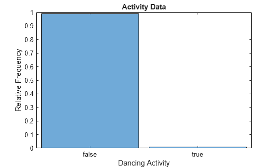
Only 1% of the observations correspond to dancing (that is, have an IsDancing value of true or 1).
Split the data into training and test sets by using the cvpartition function. Use 70% of the observations for training, and reserve 30% of the observations for testing.
rng(0,"twister") % For reproducibility
testPartition = cvpartition(data.IsDancing,Holdout=0.3);
trainingData = data(training(testPartition),:);
testData = data(test(testPartition),:);
Train and Evaluate Binary Classification Model
Use the helper function helperTrainAndTestModel to train and evaluate a support vector machine (SVM) classifier. The function uses the following code to train the classifier, which includes standardizing the predictors and using a polynomial kernel function with an appropriate scale factor.
rng(0,"twister")
mdlSVM = fitcsvm(trainingData,"IsDancing",Standardize=true, ...
    KernelFunction="polynomial",KernelScale="auto", ...
    ClassNames=[false true]);
Train the classifier using trainingData. Display the confusion matrix, compute the F1 score, precision, and recall metrics (originalMetrics), and compute the predicted class scores (originalScores) using testData. These metrics are helpful in determining the performance of the classifier when you have imbalanced data.
[originalMetrics,originalScores] = helperTrainAndTestModel(trainingData,testData,"Original");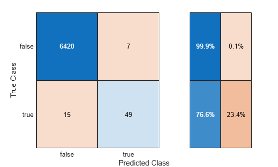
metricsTable = originalMetrics
metricsTable=1×4 table
    Technique     F1Score    Precision    Recall
    __________    _______    _________    _______

    "Original"    0.81667      0.875      0.76562
The recall value indicates that the classifier correctly classifies 76.6% of the observations corresponding to dancing. The precision value indicates that 87.5% of the observations predicted as corresponding to dancing are correct. Because the F1 score (the harmonic mean of precision and recall) is close to 1, the classifier appears to perform well on the test data.
Perform Decision Thresholding
Try to improve the classifier performance on the test data by using decision thresholding. Use cross-validation to find the optimal threshold. Cross-validation helps prevent overfitting during the tuning of the decision threshold.
Train the same type of SVM classifier using 5-fold cross-validation. For each fold, predict class scores for the observations in the fold using the SVM classifier in thresholdCVMdl trained on the remaining observations. Note that setting the ClassNames name-value argument ensures the order of the class scores in thresholdCVScores.
rng(0,"twister")
thresholdCVMdl = fitcsvm(trainingData,"IsDancing", ...
    Standardize=true,KernelFunction="polynomial", ...
    KernelScale="auto",ClassNames=[false true],KFold=5);
[~,thresholdCVScores] = kfoldPredict(thresholdCVMdl);
Optimize the decision threshold by maximizing the F1 score for the class corresponding to dancing (IsDancing=true).
trueClassCVScores = thresholdCVScores(:,2);
rocObj = rocmetrics(trainingData.IsDancing,trueClassCVScores,true, ...
    AdditionalMetrics="f1score");
[~,idx] = max(rocObj.Metrics.F1Score);
optimalThreshold = rocObj.Metrics.Threshold(idx)
optimalThreshold =
-0.2141
Use the optimal threshold to adjust the test set predicted class scores from the original SVM classifier trained using the full training data. The elements of thresholdYPred correspond to predicted IsDancing labels. When the predicted score for the class corresponding to dancing is greater than or equal to the optimal threshold, the predicted label in thresholdYPred is true.
trueClassOriginalScores = originalScores(:,2);
thresholdYPred = trueClassOriginalScores >= optimalThreshold;
Use the helper function helperComputeMetrics to display the confusion matrix and compute the F1 score, precision, and recall metrics (thresholdMetrics) for the threshold-adjusted test set predictions. In general, do not use the same data to tune the threshold and evaluate the performance of the classifier with threshold-adjusted scores.
thresholdMetrics = helperComputeMetrics(testData.IsDancing,thresholdYPred,"Thresholding");
Add the metrics to metricsTable, and compare the results.
metricsTable(2,:) = thresholdMetrics
metricsTable=2×4 table
      Technique       F1Score    Precision    Recall
    ______________    _______    _________    _______

    "Original"        0.81667       0.875     0.76562
    "Thresholding"    0.83077     0.81818     0.84375
Decision thresholding improves the F1 score and recall value for the classifier.
Perform Random Undersampling
Perform random undersampling before training the SVM classifier. Then, evaluate the performance of the classifier using the test set.
First, use the helper function helperSplitDataByClass to separate the training data into observations corresponding to dancing (dancingData) and observations corresponding to all other activities (otherActivityData). Find the difference between the number of observations in the two data sets.
[dancingData,otherActivityData,numDancing,numOtherActivity] = helperSplitDataByClass(trainingData);
numSampleDifference = numOtherActivity - numDancing;
Select the number of observations to sample (without replacement) from otherActivityData. Specifically, compute 20% of the difference between the number of observations in dancingData and otherActivityData. Reduce the number of otherActivityData observations by the resulting value.
Note that a percentageToDecrease value of 0 corresponds to the original data, and a percentageToDecrease value of 100 corresponds to perfectly balanced data. In general, choose a value that provides the proportion of observations you want from otherActivityData and dancingData.
percentageToDecrease =20; numToSample = numOtherActivity - ceil((percentageToDecrease/100)*numSampleDifference); rng(0,"twister") idx = randperm(numOtherActivity,numToSample); undersampledOtherActivity = otherActivityData(idx,:);
Combine the sampled set of observations undersampledOtherActivity with the observations in dancingData.
balancedXTrain = [undersampledOtherActivity; dancingData];
Use the helper function helperTrainAndTestModel to train the SVM classifier on the balancedXTrain data set and evaluate the classifier on the testData set. Display the confusion matrix, and compute the F1 score, precision, and recall metrics (undersampleMetrics).
undersampleMetrics = helperTrainAndTestModel(balancedXTrain,testData,"Random Undersampling");
Add the metrics to metricsTable, and compare the results.
metricsTable(3,:) = undersampleMetrics
metricsTable=3×4 table
          Technique           F1Score    Precision    Recall
    ______________________    _______    _________    _______

    "Original"                0.81667       0.875     0.76562
    "Thresholding"            0.83077     0.81818     0.84375
    "Random Undersampling"    0.83607     0.87931     0.79688
The classifier trained using random undersampling has a greater F1 score than the other two classifiers. However, the F1 score is similar to the one returned using decision thresholding.
Perform Random Oversampling
Perform random oversampling before training the SVM classifier. Then, evaluate the performance of the classifier using the test set.
Select the number of observations to sample (with replacement) from dancingData. Specifically, compute 65% of the difference between the number of observations in dancingData and otherActivityData. Select the resulting number of dancingData observations.
Note that a percentageToIncrease value of 0 corresponds to the original data, and a percentageToIncrease value of 100 corresponds to perfectly balanced data. In general, choose a value that provides the proportion of observations you want from otherActivityData and dancingData.
percentageToIncrease =65; numToSample = ceil((percentageToIncrease/100)*numSampleDifference); rng(0,"twister") idx = randi(numDancing,numToSample,1); oversampledDancingData = dancingData(idx,:);
Combine the sampled set of observations oversampledDancingData with the observations in trainingData.
balancedXTrain = [trainingData; oversampledDancingData];
Use the helper function helperTrainAndTestModel to train the SVM classifier on the balancedXTrain data set and evaluate the classifier on the testData set. Display the confusion matrix, and compute the F1 score, precision, and recall metrics (oversampleMetrics).
oversampleMetrics = helperTrainAndTestModel(balancedXTrain,testData,"Random Oversampling");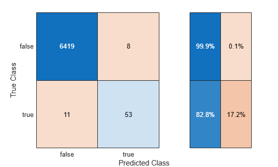
Add the metrics to metricsTable, and compare the results.
metricsTable(4,:) = oversampleMetrics
metricsTable=4×4 table
          Technique           F1Score    Precision    Recall
    ______________________    _______    _________    _______

    "Original"                0.81667       0.875     0.76562
    "Thresholding"            0.83077     0.81818     0.84375
    "Random Undersampling"    0.83607     0.87931     0.79688
    "Random Oversampling"       0.848     0.86885     0.82812
The classifier trained using random oversampling has a greater F1 score than the other classifiers.
Perform SMOTE
Use SMOTE to generate synthetic data before training the SVM classifier. Then, evaluate the performance of the classifier using the test set.
Create a smoteTabularSynthesizer object for generating synthetic data similar to the dancingData observations.
smoteMdl = smoteTabularSynthesizer(dancingData,"IsDancing");Select the number of observations to generate. Specifically, compute 65% of the difference between the number of observations in dancingData and otherActivityData. Generate the resulting number of observations.
percentageToIncrease =65; numToSample = ceil((percentageToIncrease/100)*numSampleDifference); rng(0,"twister") syntheticDancingData = synthesizeTabularData(smoteMdl,numToSample);
Use the knntest function to compare the real observations in dancingData to the synthetic observations in syntheticDancingData.
rng(0,"twister")
varNames = dancingData.Properties.VariableNames;
varNames = varNames(1:end-1);
[~,p,h] = knntest(dancingData,syntheticDancingData, ...
    VariableNames=varNames)
p =
1
h =
0
The returned test decision of h = 0 indicates that knntest fails to reject the null hypothesis that the data sets come from the same distribution at the 5% significance level.
Combine the synthetic observations syntheticDancingData with the observations in trainingData.
balancedXTrain = [trainingData; syntheticDancingData];
Use the helper function helperTrainAndTestModel to train the SVM classifier on the balancedXTrain data set and evaluate the classifier on the testData set. Display the confusion matrix, and compute the F1 score, precision, and recall metrics (smoteMetrics).
smoteMetrics = helperTrainAndTestModel(balancedXTrain,testData,"SMOTE");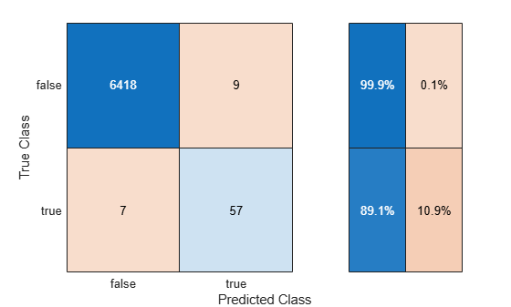
Add the metrics to metricsTable, and compare the results.
metricsTable(5,:) = smoteMetrics
metricsTable=5×4 table
          Technique           F1Score    Precision    Recall
    ______________________    _______    _________    _______

    "Original"                0.81667       0.875     0.76562
    "Thresholding"            0.83077     0.81818     0.84375
    "Random Undersampling"    0.83607     0.87931     0.79688
    "Random Oversampling"       0.848     0.86885     0.82812
    "SMOTE"                   0.87692     0.86364     0.89062
The classifier trained using SMOTE has the greatest F1 score among all the classifiers. Moreover, the classifier has high precision and recall values.
In summary, you can use decision thresholding, random undersampling, random oversampling, or SMOTE to handle class imbalance in binary classification. These techniques can lead to improvements in F1 scores, as demonstrated in this example, but do not guarantee statistical significance of the increased scores. Choose the technique that works best for your classification problem.
Helper Functions
helperLoadImbalancedData
The helperLoadImbalancedData function loads human activity data (humanactivity.mat) and returns a table. The table consists of numeric predictors (feat with featlabels as names) and a logical response variable (IsDancing) that indicates whether an activity is labeled as dancing. The function uses subsampling to guarantee that the percentage of dancing observations in the returned table is 1%.
function imbalancedData = helperLoadImbalancedData

load("humanactivity.mat","actid","feat","featlabels")

% Create binary response IsDancing with value true when actid == 5
isDancing = logical(ismember(actid,5));

% Create table with predictors and binary response
dataTable = array2table(feat);
dataTable.Properties.VariableNames = featlabels';
dataTable.IsDancing = isDancing;

% Determine how many true samples are needed for severe class imbalance
% ~1% data belongs to dancing class
numOtherActivity = sum(~dataTable.IsDancing);
numTotal = round(numOtherActivity / 0.99);
numDancing = numTotal - numOtherActivity;

% Randomly select required number of true samples
rng(0,"twister") % For reproducibility
trueIdx = find(dataTable.IsDancing);
selectedTrueIdx = trueIdx(randperm(height(trueIdx),numDancing));

% Combine all false samples with sampled true samples
selectedIdx = [find(~dataTable.IsDancing); selectedTrueIdx];
dataTable = dataTable(selectedIdx,:);

% Shuffle the data
imbalancedData = dataTable(randperm(height(dataTable)),:);
end
helperTrainAndTestModel
The helperTrainAndTestModel function takes a table of training data (trainingData) containing the IsDancing response variable and creates a binary SVM classifier. The function uses the table of test data (testData) to compute and return a matrix of predicted class scores (mdlScores). The function also uses the helper function helperComputeMetrics to display the confusion matrix and compute the F1 score, precision, and recall metrics (metricsTable) on the test data. The string scalar techniqueName specifies the first value in the table metricsTable.
function [metricsTable,mdlScores] = helperTrainAndTestModel( ...
    trainingData,testData,techniqueName)

% Train model
rng(0,"twister")
mdlSVM = fitcsvm(trainingData,"IsDancing",Standardize=true, ...
    KernelFunction="polynomial",KernelScale="auto", ...
    ClassNames=[false true]);

% Compute metrics using test data
[mdlPreds,mdlScores] = predict(mdlSVM,testData);
metricsTable = helperComputeMetrics(testData.IsDancing,mdlPreds,techniqueName);
end
helperComputeMetrics
The helperComputeMetrics function takes a logical vector of observed labels (YTrue) and a logical vector of predicted labels (YPred) and returns a table of metrics (metricsTable). The table includes the F1 score, precision, and recall values for the true class. The string scalar techniqueName specifies the first value in the table. The function additionally generates a confusion matrix that includes the true positive rates and false positive rates in the row summary.
function metricsTable = helperComputeMetrics(YTrue,YPred,techniqueName)

confusionchart(YTrue,YPred,RowSummary="row-normalized")

% Validate that input sizes match
if length(YTrue) ~= length(YPred)
    error("YTrue and YPred must be of the same length.");
end

% Compute confusion matrix
TP = sum((YTrue == true) & (YPred == true));
FP = sum((YTrue == false) & (YPred == true));
FN = sum((YTrue == true) & (YPred == false));

% Compute precision - how many predicted as positive are actually positive
if TP + FP == 0
    precision = 0;
else
    precision = TP / (TP + FP);
end

% Compute recall - how many of actual positive were correctly identified
if TP + FN == 0
    recall = 0;
else
    recall = TP / (TP + FN);
end

% Compute F1 score
if precision + recall == 0
    F1 = 0;
else
    F1 = 2 * (precision * recall) / (precision + recall);
end

varnames = ["Technique","F1Score","Precision","Recall"];
metricsTable = table(techniqueName,F1,precision,recall, ...
    VariableNames=varnames);
end
helperSplitDataByClass
The helperSplitDataByClass function takes a table of sample data (XTrain) and splits the data according to the IsDancing logical vector in the table. The function returns two tables: dancingData, which contains the observations that correspond to dancing, and otherActivityData, which contains the remaining observations. The function also returns the integer scalars numDancing and numOtherActivity, which contain the number of observations in dancingData and otherActivityData, respectively.
function [dancingData,otherActivityData,numDancing,numOtherActivity] = ...
    helperSplitDataByClass(XTrain)
dancingData = XTrain(XTrain.IsDancing, :);
otherActivityData = XTrain(~XTrain.IsDancing, :);
numDancing = height(dancingData);
numOtherActivity = height(otherActivityData);
end
See Also
fitcsvm | smoteTabularSynthesizer | synthesizeTabularData | confusionchart | rocmetrics | randperm | randi