Gamma Distribution
Overview
The gamma distribution is a two-parameter family of curves. The gamma distribution models sums of exponentially distributed random variables and generalizes both the chi-square and exponential distributions.
Statistics and Machine Learning Toolbox™ offers several ways to work with the gamma distribution.
Create a probability distribution object
GammaDistributionby fitting a probability distribution to sample data (fitdist) or by specifying parameter values (makedist). Then, use object functions to evaluate the distribution, generate random numbers, and so on.Work with the gamma distribution interactively by using the Distribution Fitter app. You can export an object from the app and use the object functions.
Use distribution-specific functions (
gamcdf,gampdf,gaminv,gamlike,gamstat,gamfit,gamrnd,randg) with specified distribution parameters. The distribution-specific functions can accept parameters of multiple gamma distributions.Use generic distribution functions (
cdf,icdf,pdf,random) with a specified distribution name ("Gamma") and parameters.
Parameters
The gamma distribution uses the following parameters.
| Parameter | Description | Support |
|---|---|---|
a
| Shape | a > 0 |
b | Scale | b > 0 |
The standard gamma distribution has unit scale.
The sum of two gamma random variables with shape parameters a1 and a2 both with scale parameter b is a gamma random variable with shape parameter a = a1 + a2 and scale parameter b.
Parameter Estimation
The likelihood function is the probability density
function (pdf) viewed as a function of the parameters. The maximum
likelihood estimates (MLEs) are the parameter estimates that
maximize the likelihood function for fixed values of
x.
The maximum likelihood estimators of a and b for the gamma distribution are the solutions to the simultaneous equations
where is the sample mean for the sample x1,
x2, …,
xn, and Ψ is the digamma function psi.
To fit the gamma distribution to data and find parameter estimates, use
gamfit, fitdist, or mle. Unlike
gamfit and mle, which return
parameter estimates, fitdist returns the fitted probability
distribution object GammaDistribution. The object
properties a and b store the parameter
estimates.
For an example, see Fit Gamma Distribution to Data.
Probability Density Function
The pdf of the gamma distribution is
for x ≥ 0, where Γ( · ) is the Gamma function, and a and b are the shape parameters.
For an example, see Compute Gamma Distribution pdf.
Cumulative Distribution Function
The cumulative distribution function (cdf) of the gamma distribution is
for x ≥ 0. The result p is the probability that a single observation from the gamma distribution with parameters a and b falls in the interval [0 x].
For an example, see Compute Gamma Distribution cdf.
The gamma cdf is related to the incomplete gamma function gammainc by
Inverse Cumulative Distribution Function
The inverse cumulative distribution function (icdf) of the gamma distribution in terms of the gamma cdf is
where
The result x is the value such that an observation from the gamma distribution with parameters a and b falls in the range [0 x] with probability p.
The preceding integral equation has no known analytical solution. gaminv uses an iterative approach
(Newton's method) to converge on the solution.
Descriptive Statistics
The mean of the gamma distribution is ab.
The variance of the gamma distribution is ab2.
Examples
Fit Gamma Distribution to Data
Generate a sample of 100 gamma random numbers with shape 3 and scale 5.
x = gamrnd(3,5,100,1);
Fit a gamma distribution to data using fitdist.
pd = fitdist(x,'gamma')pd =
GammaDistribution
Gamma distribution
a = 2.7783 [2.1374, 3.61137]
b = 5.73438 [4.30198, 7.64372]
fitdist returns a GammaDistribution object. The intervals next to the parameter estimates are the 95% confidence intervals for the distribution parameters.
Estimate the parameters a and b using the distribution functions.
[muhat,muci] = gamfit(x) % Distribution specific functionmuhat = 1×2
2.7783 5.7344
muci = 2×2

    2.1374    4.3020
    3.6114    7.6437
[muhat2,muci2] = mle(x,'distribution','gamma') % Generic function
muhat2 = 1×2

    2.7783    5.7344
muci2 = 2×2

    2.1374    4.3020
    3.6114    7.6437
Compute Gamma Distribution pdf
Compute the pdfs of the gamma distribution with several shape and scale parameters.
x = 0:0.1:50;
y1 = gampdf(x,1,10);
y2 = gampdf(x,3,5);
y3 = gampdf(x,6,4);
Plot the pdfs.
figure;
plot(x,y1)
hold on
plot(x,y2)
plot(x,y3)
hold off
xlabel('Observation')
ylabel('Probability Density')
legend('a = 1, b = 10','a = 3, b = 5','a = 6, b = 4')

Compute Gamma Distribution cdf
Compute the cdfs of the gamma distribution with several shape and scale parameters.
x = 0:0.1:50;
y1 = gamcdf(x,1,10);
y2 = gamcdf(x,3,5);
y3 = gamcdf(x,6,4);
Plot the cdfs.
figure;
plot(x,y1)
hold on
plot(x,y2)
plot(x,y3)
hold off
xlabel('Observation')
ylabel('Cumulative Probability')
legend('a = 1, b = 10','a = 3, b = 5','a = 6, b = 4',"Location","northwest")

Compare Gamma and Normal Distribution pdfs
The gamma distribution has the shape parameter and the scale parameter . For a large , the gamma distribution closely approximates the normal distribution with mean and variance .
Compute the pdf of a gamma distribution with parameters a = 100 and b = 5.
a = 100;
b = 5;
x = 250:750;
y_gam = gampdf(x,a,b);
For comparison, compute the mean, standard deviation, and pdf of the normal distribution that gamma approximates.
mu = a*b
mu =
500
sigma = sqrt(a*b^2)
sigma =
50
y_norm = normpdf(x,mu,sigma);
Plot the pdfs of the gamma distribution and the normal distribution on the same figure.
plot(x,y_gam,'-',x,y_norm,'-.')
title('Gamma and Normal pdfs')
xlabel('Observation')
ylabel('Probability Density')
legend('Gamma Distribution','Normal Distribution')
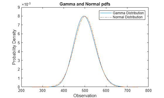
The pdf of the normal distribution approximates the pdf of the gamma distribution.
Related Distributions
Beta Distribution — The beta distribution is a two-parameter continuous distribution that has parameters a (first shape parameter) and b (second shape parameter). If X1 and X2 have standard gamma distributions with shape parameters a1 and a2 respectively, then has a beta distribution with shape parameters a1 and a2.
Chi-Square Distribution — The chi-square distribution is a one-parameter continuous distribution that has parameter ν (degrees of freedom). The chi-square distribution is equal to the gamma distribution with 2a = ν and b = 2.
Exponential Distribution — The exponential distribution is a one-parameter continuous distribution that has parameter μ (mean). The exponential distribution is equal to the gamma distribution with a = 1 and b = μ. The sum of k exponentially distributed random variables with mean μ is the gamma distribution with parameters a = k and μ = b.
Nakagami Distribution — The Nakagami distribution is a two-parameter continuous distribution with shape parameter µ and scale parameter ω. If x has a Nakagami distribution, then x2 has a gamma distribution with a = μ and ab = ω.
Normal Distribution — The normal distribution is a two-parameter continuous distribution that has parameters μ (mean) and σ (standard deviation). When a is large, the gamma distribution closely approximates a normal distribution with μ = ab and σ2 = ab2. For an example, see Compare Gamma and Normal Distribution pdfs.
References
[1] Abramowitz, Milton, and Irene A. Stegun, eds. Handbook of Mathematical Functions: With Formulas, Graphs, and Mathematical Tables. 9. Dover print.; [Nachdr. der Ausg. von 1972]. Dover Books on Mathematics. New York, NY: Dover Publ, 2013.
[2] Evans, Merran, Nicholas Hastings, and Brian Peacock. Statistical Distributions. 2nd ed. New York: J. Wiley, 1993.
[3] Hahn, Gerald J., and Samuel S. Shapiro. Statistical Models in Engineering. Wiley Classics Library. New York: Wiley, 1994.
[4] Lawless, Jerald F. Statistical Models and Methods for Lifetime Data. 2nd ed. Wiley Series in Probability and Statistics. Hoboken, N.J: Wiley-Interscience, 2003.
[5] Meeker, William Q., and Luis A. Escobar. Statistical Methods for Reliability Data. Wiley Series in Probability and Statistics. Applied Probability and Statistics Section. New York: Wiley, 1998.
[6] Marsaglia, George, and Wai Wan Tsang. “A Simple Method for Generating Gamma Variables.” ACM Transactions on Mathematical Software 26, no. 3 (September 1, 2000): 363–72. https://doi.org/10.1007/978-1-4613-8643-8.
See Also
GammaDistribution | gamcdf | gampdf | gaminv | gamlike | gamstat | gamfit | gamrnd | randg | makedist | fitdist