DOE Explorer
R2026bDescription
The DOE Explorer app lets you design systematic experiments and analyze response data using design of experiments (DOE) algorithms.
Using this app, you can:
Generate a full factorial, fractional factorial, D-optimal, or response surface design using continuous and categorical factors with default or custom factor levels.
Import an existing design and response data from a file or the MATLAB® workspace.
Fit a model to the response data using ordinary or stepwise linear regression.
Analyze the effects of factors on the responses and factor interactions using the following plots: standardized effects, estimated effects, residuals, estimated interactions, and slice plots.
Required Products
MATLAB
Statistics and Machine Learning Toolbox™
Open the DOE Explorer App
MATLAB Toolstrip: On the Apps tab, under Math, Statistics and Optimization, click the app icon.
MATLAB command prompt: Enter
doeExplorer.
Parameters
Design Tab
Click New to start a new experiment. This action deletes the current design table, response data, linear regression model, and plots.
To import a design table and response data into the app, click Import Design Table and select one of these options:
From Workspace — Select a table variable in the MATLAB workspace to import. Each table row contains a run, and each table variable contains settings for a factor. A table variable can optionally contain response data.
From File — Select a text file or spreadsheet file to import. The app opens the Import Tool. Each row contains a run, and each variable (column) contains a factor. A variable can optionally contain response data. Select the runs and variables to import, and click Import Selection.
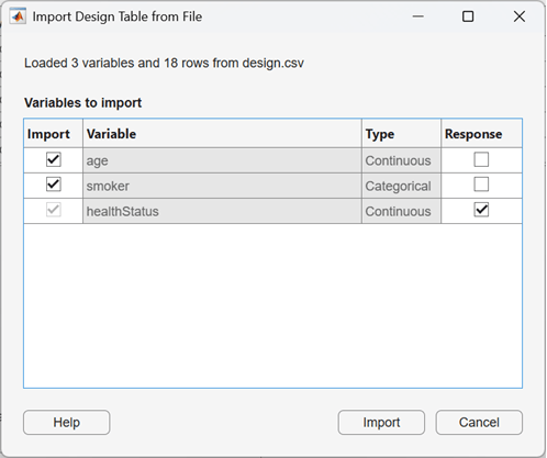
In the dialog box, select the variables to import as factors. To import response data, select a variable in the Response column. Click Import to import the design table.
To set up a design, choose one of the following design types.
| Design | Description | More Information |
|---|---|---|
| Full Factorial | Contains a run for every possible combination of factor levels | Full Factorial Designs |
| Fractional Factorial | Contains a fraction of all possible runs. Use a fractional factorial design to screen two-level factors when you know that higher order interactions are negligible. | Fractional Factorial Designs |
| D-Optimal | Use this design type when you want to incorporate irregular constraints or a nonstandard model equation. | D-Optimal Designs |
| Response Surface | Use this design type when you know there is a nonlinear relationship between the factors and the response. You can choose a central composite or Box–Behnken design. | Response Surface Designs |
To fit a model to the response data using the default regression model, click Model and select one of the options described below. This button is not available until you generate or import a design table and enter or import response data. For a response surface design, the default model is quadratic. For a D-optimal design, you specify the default model in the Setup Tab. For all other design types, the default model is linear.
Linear Regression — Fit a linear model to the response data using ordinary linear regression. The app displays the results in the Fit Summary Tab. Specify a different model using the Fit Options panel on the right side of the tab. For more information about ordinary linear regression, see
fitlm.Stepwise Linear Regression — Fit a model to the response data using stepwise linear regression. To specify stepwise regression options, use the Fit Options panel on the right side of the Fit Summary tab. For more information about stepwise linear regression, see
stepwiselm.
If you already fit a regression model, and you select Linear Regression or Stepwise Linear Regression, the app deletes the current fit and performs a new fit with the default model and default fit options.
For more information about linear regression models, see What Is a Linear Regression Model?.
Setup Tab
Use the Add Factor and Remove Selected Factor buttons to add and remove factors from the design. These buttons are not available when you import a design table into the app. You can adjust entries in the following table columns:
Factor Name — Enter a label for the factor.
Type — Select
Continuousfor a factor with ordinal, numeric level values. SelectCategoricalfor a factor with nominal level values (see Categorical Factors). The Type column is not displayed for a response surface design, which contains only continuous factors. You cannot adjust the factor type when you import a design table.The rightmost columns in the table depend on the design type.
Imported design table — The Levels column is not displayed. You cannot adjust the level values in an imported design table.
Full factorial or D-optimal design — Enter the level values of each factor in the Levels column as a comma-separated list. Alternatively, you can assign evenly spaced levels within a specified range for a continuous factor. Select a factor and click the Modify levels button above the table. In the Modify Factor Levels dialog box, specify the Lower Bound and Upper Bound values, and enter the number of levels to assign within the bounds in the Number of Levels box.
Fractional factorial design — Enter the first and second level values for each factor in the First Level and Second Level columns, respectively. The app supports only two-level fractional factorial designs.
Response surface design — Enter the lower and upper level bound values in the Lower Level Bound and Upper Level Bound columns, respectively. The app assigns the level values for each design run within the level bounds according to the response surface design type.
A continuous factor must have numeric level values. The level values of a categorical factor can contain any alphanumeric character.
Enter a label for the response. The default label is Response.
The app uses the response label in the linear regression model equation display and in
the Design Table Tab.
The options in this section depend on the design type that you select in the Designs gallery. When you finish setting design options, click Generate Design Table at the bottom of the Setup tab to generate the design table. You cannot set any design options when you import a design table.
Full factorial designs — You cannot set any design options. The app displays the number of design runs in the Design Characteristics section.
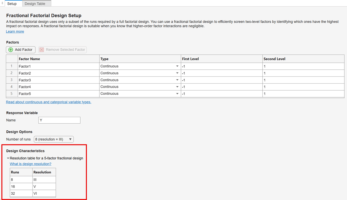
Fractional factorial designs — Select the number of runs in the design and the corresponding resolution. The resolution depends on the number of factors and runs. The Design Characteristics section shows the resolution table and confounding pattern for the selected design options. For more information, see Fractional Factorial Design Resolution and Confounding.
D-optimal designs — You can set the following options:
Number of runs— Enter the number of runs in the design. The default value is20.Exchange method— Select either theCoordinate(default) orRowexchange algorithm for generating the design. For more information, see the Algorithms sections ofcordexchandrowexch.Avoid duplicate runs— When you select this option, the app adds additional levels for any continuous factors, as needed, to avoid duplicate rows in the design.Max number of start runs— Specify the number of designs to generate from different start runs. The default value is1. The app chooses the design with the least amount of covariance between the coefficient estimates for the specified regression model equation.Max iterations per try— Specify the maximum number of iterations per start run for the algorithm that generates the design runs. The default value is10.Model— Specify the regression model for the D-optimal design. The default setting isLinear. For more information, see Regression Model Types. The app generates a design that minimizes the covariance between the estimated model coefficients. This model becomes the default model for the linear regression fit.
Response surface designs — Select one of the following types:
Central Composite(default) — When you select this option, you can also specify the central composite type, the number of center points, and the fractional design index. For more information, see Central Composite Designs.Box-Behnken— When you have three or four factors, a Box–Behnken design requires fewer runs than a central composite design. A Box–Behnken design is also rotatable, meaning that the prediction variance depends only on the distance of the design point from the center of the design. You can enter the number of center points for the design or use the defaultAutosetting to choose the number of center points automatically based on the number of factors. For more information, see Box–Behnken Designs.
Design Table Tab
The design table contains a row for each run in the experiment, and columns with
level values for each factor. The rightmost column contains the response values. You can
enter or adjust the response values, and import responses using the From
Workspace or From File buttons located above the table
(see Import response data). When you fit a
regression model to the response data, the app ignores any run in the table that has a
missing or NaN response value.
Select this option to display continuous factor levels in coded units. For more information, see Coded Units. This setting does not affect the linear regression fit or plots.
To import response data for the design runs, click one of the following buttons:
From Workspace — Select a workspace variable that contains the response data. The variable must be a numeric row or column vector with length equal to the number of runs in the design.
From File — Select a text or spreadsheet file in the dialog box and click Open. In the Import Tool window, select a single column that contains the response data. The number of rows in the selection must equal the number of runs in the design.
Fit Summary Tab
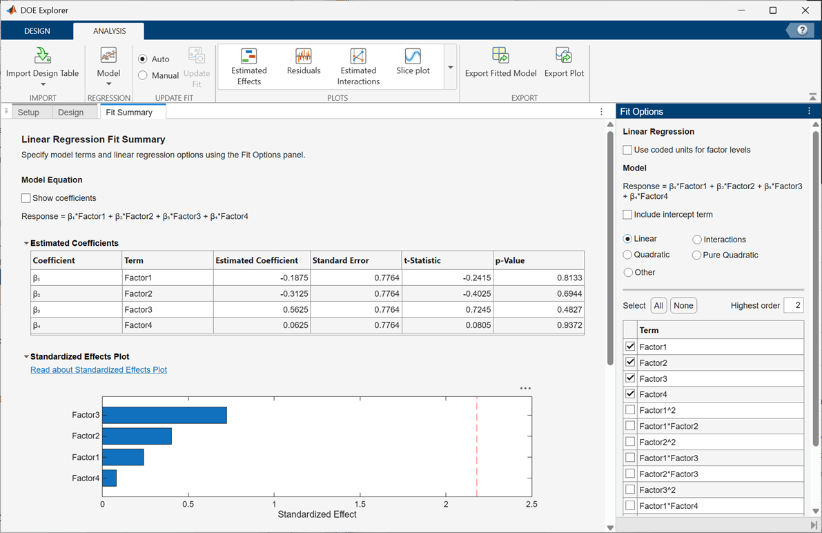
The estimated coefficients table contains the following columns for the linear regression model fit:
Coefficient — Coefficient label
Term — Model term
Estimated Value — Estimated coefficient value
Standard Error — Standard error of the coefficient estimate
t-Statistic — t-statistic for a two-sided test with the null hypothesis that the coefficient value is zero
p-Value — p-value for the t-statistic
For more information about linear regression model fit coefficients, see
fitlm
and stepwiselm.
The standardized effects plot is a Pareto (bar) chart of the absolute t-statistic values for the terms in the regression model. Use the plot to determine which terms have a significant effect on the response. Any bar that crosses the red dashed line is statistically significant at the 95% confidence level.
At each step in the stepwise linear regression algorithm, the app searches for terms
to add to the model or remove from the model, based on the Import Tool. Each row in the Step History table lists the
action taken (Start, Add, or
Remove) in the Action column, and the terms in
the model equation at the end of the step in the Terms column. When
you select SSE (sum of squares) for Criterion
(the default) in the Fit Options panel, the table displays columns
containing the F-statistic and the corresponding
p-value to test models with and without a potential term at each
step. For all other Criterion options, the table displays a column
containing the criterion value.
For more information about stepwise regression, see the Algorithms
section of the stepwiselm function reference page.
The table contains ANOVA (analysis of variance) statistics for each term in the regression model (except the intercept) and an error term. The table has the following columns:
Variability Source — Variability term.
Sum of Squares — Sum of squares. The app uses a hierarchical model to compute the sum of squares.
DF — Degrees of freedom.
Mean Square — Mean square, which is the ratio
Sum of Squares/DF. The mean square of the error term is the mean squared error (MSE).F-Statistic — F-statistic value to test the null hypothesis that the corresponding coefficient is zero. The F-statistic is the ratio
Mean Square/ MSE.p-Value — Probability that the F-statistic can take a value larger than the computed test-statistic value. The app derives the probability from the cumulative distribution function of the F-distribution.
For more information about ANOVA, see anova.
The goodness-of-fit table contains the following statistics. The rightmost column in
the table below lists the corresponding property of the LinearModel object that you can create using the Export Fitted
Model button in the Analysis tab.
| Name | Description | LinearModel Object Property |
|---|---|---|
| Number of observations | Number of responses | NumObservations
|
| Error degrees of freedom | n minus k, where n is the number of responses, and k is the number of terms in the model, including the intercept | DFE
|
| Root mean squared error | Square root of the mean squared error, which estimates the standard deviation of the error distribution |
RMSE |
| R-squared | Coefficient of determination |
Rsquared.Ordinary |
| Adjusted R-squared | Adjusted coefficient of determination | Rsquared.Adjusted
|
| F-statistic vs. constant model | Test statistic for the F-test on the linear regression model, which tests whether the model fits significantly better than a degenerate model consisting of only a constant term | ModelFitVsNullModel.Fstat |
| p-Value | p-value for the F-test on the model | ModelFitVsNullModel.Pvalue |
Use the settings in this panel to specify options for ordinary and stepwise linear regression and model equation terms. For a description of the regression fit results, see Fit Summary Tab.
Select Use coded units for factor levels to use coded units for continuous factor levels in the regression fit and plots. For more information, see Coded Units.
Select Use coded units for factor levels to use coded units for continuous factor levels in the regression fit and plots. For more information, see Coded Units.
Enter a positive integer in the Maximum steps box to set
the maximum number of iteration steps. Select the Unlimited
check box or enter Inf (the default) to run the algorithm until
no single step improves the model.
For ordinary linear regression, you can select a set of terms for the linear regression model (see Regression Model Types). Select Include intercept term to include an intercept term. You can also select individual model terms using the check boxes in the terms table. By default, the app displays only terms up to second order. To display higher order terms, enter an integer value in the Highest order box.
For stepwise linear regression, you can set the following options:
Initial set of terms — Specify the initial set of model terms for the stepwise regression.
Smallest set of terms— Select the smallest set of terms that cannot be removed from the model.
Largest set of terms— Select the largest set of terms that can be included in the model.
The following options are available for stepwise regression:
Criterion — Select one of the following criteria to add or remove model terms:
SSE (sum of squared error)— p-value for an F-test of the change in the sum of squared error that results from adding or removing the termAIC (Akaike information criterion)— Change in the value of the Akaike information criterion (AIC)BIC (Bayesian information criterion)— Change in the value of the Bayesian information criterion (BIC)R-squared— Increase in the value of R2Adjusted R-squared— Increase in the value of adjusted R2
Threshold to add term — Specify the threshold for the criterion to add a term to the model, as described in this table. The default value is
0.05.Criterion Decision SSEIf the p-value of the F-statistic is less than the threshold value, add the term to the model. AICIf the change in the AIC of the model is less than the threshold value, add the term to the model. BICIf the change in the BIC of the model is less than the threshold value, add the term to the model. RsquaredIf the increase in the R-squared value of the model is greater than the threshold value, add the term to the model. AdjRsquaredIf the increase in the adjusted R-squared value of the model is greater than the threshold value, add the term to the model. To prevent the app from adding terms to the model during the stepwise regression, specify the threshold as a value that the app cannot achieve.
When Criterion is
SSE,AIC, orBIC, specify the threshold as–Inf.When Criterion is
RsquaredorAdjRsquared, specify the threshold asInf.
Threshold to remove term — Specify the threshold for the criterion to remove a term from the model, as described in this table. The default value is
0.1Criterion Decision SSEIf the p-value of the F-statistic is greater than the threshold value, remove the term from the model. AICIf the change in the AIC of the model is greater than the threshold value, remove the term from the model. BICIf the change in the BIC of the model is greater than the threshold value, remove the term from the model. RsquaredIf the increase in the R-squared value of the model is less than the threshold value, remove the term from the model. AdjRsquaredIf the increase in the adjusted R-squared value of the model is less than the threshold value, remove the term from the model. At each step, the app also checks whether a term is redundant (linearly dependent) with other terms in the current model. When any term is linearly dependent with other terms in the current model, the app removes the redundant term, regardless of the criterion value.
To prevent the app from removing model terms during the stepwise regression, specify the threshold as a value that the app cannot achieve.
When Criterion is
SSE,AIC, orBIC, specify the threshold asInf.When Criterion is
RsquaredorAdjRsquared, specify the threshold as–Inf.
For more information about stepwise regression, see the Algorithms section of the
stepwiselmfunction reference page.
Plot Gallery
This plot displays the estimated main effect on the response from changing each
factor value, averaging out the effects of the other factors. A horizontal line through
an effect value indicates the 95% confidence interval for the effect value. To display
an estimated effects plot, you must generate or import a design and enter or import
response data. Then use the Model button in the toolstrip to fit a
regression model with at least one term that includes a factor. For more information,
see the Main Effect section of the
plotEffects function reference page.
Click the Residuals button to display a plot of model residuals (comparison statistics between predicted and observed response values). To display a residuals plot, you must first fit a regression model to the response data using the Model button in the toolstrip. You can select the residuals plot type and the residual type using the following options in the Residuals Plot tab.
Select one of the following residuals plot types:
Residual vs. run number— Residual versus run number.Observed vs. fitted— Observed response versus predicted response. This plot includes a dotted reference line of y = x. Each residual is represented by the vertical distance from the corresponding observed response value to the reference line.Residual vs. fitted— Residual versus predicted response.Residual vs. lagged residual— Residuals vs. lagged residuals (r(n) vs. r(n – 1)), where r(n) is the residual for run n.Normal probability— Normal probability plot of residuals. For details, seeprobplot.Histogram of residuals— Histogram of residuals using probability density function scaling. The area of each bar is the relative number of responses. The sum of the bar areas is equal to 1.Symmetry— Symmetry plot of residuals around their median (residuals in the upper tail minus median vs. median minus residuals in the lower tail). This plot includes a dotted reference line of y = x to examine the symmetry of the residuals.
For more information on residuals plot types, see plotResiduals.
Select one of the following residual types:
Raw— Observed minus fitted response valuesPearson— Raw residuals divided by the root mean squared error (RMSE)Standardized— Raw residuals divided by their estimated standard deviationStudentized— Raw residuals divided by an independent (delete-1) estimate of their standard deviation
For more information about residual types, see Residuals.
To display an estimated interactions plot, you must first use the
Model button in the toolstrip to fit a regression model that
contains interaction terms. Select Plot matrix (the default) to
plot all factor combinations, or Single plot to plot a single pair
of factors. An estimated interactions plot displays the conditional effect of one
predictor on the response, given a specific value of another factor. For more
information, see the plotInteraction reference page.
To display a slice plot, you must first use the Model button in the toolstrip to fit a regression model. Click the Slice button to create a figure containing one or more plots, each representing a slice through the fitted linear regression surface. Each plot shows the fitted response values as a function of a single factor, with the other factor values held constant. Click Select Factors to select the factors to plot. Select Show confidence intervals (the default) to display confidence intervals. You can select the following confidence interval options:
Simultaneous bounds — Select this option (the default) to compute confidence bounds for the curve of the response values using Scheffé's method. The range between the upper and lower confidence bounds contains the curve consisting of true response values with 95% confidence.
Clear this check box to compute confidence bounds for the response value at each observation. The confidence interval for a response value at a specific factor value contains the true response value with 95% confidence.
With simultaneous bounds, the entire curve of true response values is within the bounds at high confidence. By contrast, nonsimultaneous bounds require only the response value at a single factor value to be within the bounds at high confidence. Therefore, simultaneous bounds are wider than nonsimultaneous bounds.
Bounds Type — You can select one of the following bounds types:
Curve (default) — The app predicts confidence bounds for the fitted responses.
Observation — The app predicts confidence bounds for the response observations.
The regression model for the factors X and the response y has the form
y = f(X) + ε,
where f is a function of X and ε is a random noise term. The bounds for Observation are wider than the bounds for Curve due to the additional variability of the noise term.
For more information about slice plots, see the plotSlice
function reference page.
Programmatic Use
Limitations
Supported Design Types
In DOE Explorer, you can generate Full Factorial Designs, Fractional Factorial Designs, Response Surface Designs, and D-Optimal Designs. You can
also import your own design table and responses from the MATLAB workspace or a file into the
app (see Import Design Table). To generate Taguchi Designs and mixture experiment
designs, use the command line functions taguchiDOE and
mixtureDOE,
respectively.
More About
In a fractional factorial design, you select a subset of experimental treatments based on an evaluation (or assumption) of which factors and interactions have the most significant effects on the response. A main effect is the impact a factor has on the response, averaged over all the levels of the other factors. A process contains an interaction when the impact of one factor depends on the level value of one or more other factors. After you select the main effects and interactions to include, your experiment design should be able to separate them. In particular, significant effects should not be confounded, that is, the measurement of one effect should not depend on the measurement of another effect. The resolution of a fractional factorial design (indicated by a Roman numeral) describes the amount of confounding that is present.
If only main effects are significant in the process, you can use a resolution III (Plackett–Burman) fractional factorial design. Otherwise, you can specify which significant interactions to consider by using a higher resolution design, at the cost of adding more runs. In a fractional factorial design of resolution R, no n-factor interaction is confounded with any other effect containing less than R – n factors. Therefore, a resolution III design does not confound main effects with one another, but might confound them with two-way interactions. A resolution IV design does not confound main effects with one another, or main effects with two-way interactions, but might confound two-way interactions with one another.
You can view a resolution table in the Design Characteristics section of the Setup tab. The table values assume a linear experiment model. To specify the number of runs and design resolution, select an option from the list in the Design Options section.
You can view a confounding pattern table for a linear model in the Design Characteristics section of the Setup tab.
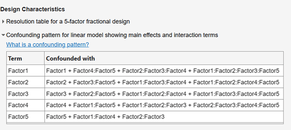
The first column in the table contains a term in the model specification, and the second
column contains the interaction terms. The table entries depend on the number of runs and
factors in the design, and the experimental model. For example, if the term
Factor1 has an interaction term
Factor2:Factor3:Factor4:Factor5, then in a linear model, you cannot
estimate the term and the interaction term at the same time. The estimated effect for
Factor1 is a combination of the effects of Factor1
and Factor2:Factor3:Factor4:Factor5.
Version History
Introduced in R2026b

