predictLifetime

Compute cumulative lifetime PD, marginal PD, and survival probability

Since R2020b

Syntax

LifeTimePredictedPD = predictLifetime(pdModel,data)

LifeTimePredictedPD = predictLifetime(___,Name,Value)

Description

LifeTimePredictedPD = predictLifetime(pdModel,data) computes the cumulative lifetime probability of default (PD), marginal PD, and survival probability.

example

LifeTimePredictedPD = predictLifetime(___,Name,Value) specifies options using one or more name-value pair arguments in addition to the input arguments in the previous syntax.

Examples

collapse all

Use Probit Lifetime PD Model to Predict Lifetime PD

Open Live Script

This example shows how to use fitLifetimePDModel to fit data with a Probit model and then predict the lifetime probability of default (PD).

Load Data

Load the credit portfolio data.

load RetailCreditPanelData.mat
disp(head(data))

    ID    ScoreGroup    YOB    Default    Year
    __    __________    ___    _______    ____

    1      Low Risk      1        0       1997
    1      Low Risk      2        0       1998
    1      Low Risk      3        0       1999
    1      Low Risk      4        0       2000
    1      Low Risk      5        0       2001
    1      Low Risk      6        0       2002
    1      Low Risk      7        0       2003
    1      Low Risk      8        0       2004

disp(head(dataMacro))

    Year     GDP     Market
    ____    _____    ______

    1997     2.72      7.61
    1998     3.57     26.24
    1999     2.86      18.1
    2000     2.43      3.19
    2001     1.26    -10.51
    2002    -0.59    -22.95
    2003     0.63      2.78
    2004     1.85      9.48

Join the two data components into a single data set.

data = join(data,dataMacro);
disp(head(data))

    ID    ScoreGroup    YOB    Default    Year     GDP     Market
    __    __________    ___    _______    ____    _____    ______

    1      Low Risk      1        0       1997     2.72      7.61
    1      Low Risk      2        0       1998     3.57     26.24
    1      Low Risk      3        0       1999     2.86      18.1
    1      Low Risk      4        0       2000     2.43      3.19
    1      Low Risk      5        0       2001     1.26    -10.51
    1      Low Risk      6        0       2002    -0.59    -22.95
    1      Low Risk      7        0       2003     0.63      2.78
    1      Low Risk      8        0       2004     1.85      9.48

Partition Data

Separate the data into training and test partitions.

nIDs = max(data.ID);
uniqueIDs = unique(data.ID);

rng('default'); % for reproducibility
c = cvpartition(nIDs,'HoldOut',0.4);

TrainIDInd = training(c);
TestIDInd = test(c);

TrainDataInd = ismember(data.ID,uniqueIDs(TrainIDInd));
TestDataInd = ismember(data.ID,uniqueIDs(TestIDInd));

Create a Probit Lifetime PD Model

Use fitLifetimePDModel to create a Probit model using the training data.

pdModel = fitLifetimePDModel(data(TrainDataInd,:),"Probit",...
    'AgeVar','YOB',...
    'IDVar','ID',...
    'LoanVars','ScoreGroup',...
    'MacroVars',{'GDP','Market'},...
    'ResponseVar','Default');
disp(pdModel)

  Probit with properties:

            ModelID: "Probit"
        Description: ""
    UnderlyingModel: [1x1 classreg.regr.CompactGeneralizedLinearModel]
              IDVar: "ID"
             AgeVar: "YOB"
           LoanVars: "ScoreGroup"
          MacroVars: ["GDP"    "Market"]
        ResponseVar: "Default"

Display the underlying model.

disp(pdModel.Model)

Compact generalized linear regression model:
    probit(Default) ~ 1 + ScoreGroup + YOB + GDP + Market
    Distribution = Binomial

Estimated Coefficients:
                               Estimate        SE         tStat       pValue   
                              __________    _________    _______    ___________

    (Intercept)                  -1.6267      0.03811    -42.685              0
    ScoreGroup_Medium Risk      -0.26542      0.01419    -18.704     4.5503e-78
    ScoreGroup_Low Risk         -0.46794     0.016364    -28.595     7.775e-180
    YOB                         -0.11421    0.0049724    -22.969    9.6208e-117
    GDP                        -0.041537     0.014807    -2.8052      0.0050291
    Market                    -0.0029609    0.0010618    -2.7885      0.0052954


388097 observations, 388091 error degrees of freedom
Dispersion: 1
Chi^2-statistic vs. constant model: 1.85e+03, p-value = 0

Predict Lifetime PD on Training and Test Data

Use the predictLifetime function to get lifetime PDs on the training or the test data. To get conditional PDs, use the predict function. For model validation, use the modelDiscrimination and modelCalibration functions on the training or test data.

DataSetChoice = "Testing";
if DataSetChoice=="Training"
    Ind = TrainDataInd;
else
    Ind = TestDataInd;
end

% Predict lifetime PD
PD = predictLifetime(pdModel,data(Ind,:));
head(data(Ind,:))

    ID    ScoreGroup     YOB    Default    Year     GDP     Market
    __    ___________    ___    _______    ____    _____    ______

    2     Medium Risk     1        0       1997     2.72      7.61
    2     Medium Risk     2        0       1998     3.57     26.24
    2     Medium Risk     3        0       1999     2.86      18.1
    2     Medium Risk     4        0       2000     2.43      3.19
    2     Medium Risk     5        0       2001     1.26    -10.51
    2     Medium Risk     6        0       2002    -0.59    -22.95
    2     Medium Risk     7        0       2003     0.63      2.78
    2     Medium Risk     8        0       2004     1.85      9.48

Predict Lifetime PD on New Data

Lifetime PD models are used to make predictions on existing loans. The predictLifetime function requires projected values for both the loan and macro predictors for the remainder of the life of the loan.

The DataPredictLifetime.mat file contains projections for two loans and also for the macro variables. One loan is three years old at the end of 2019, with a lifetime of 10 years, and the other loan is six years old with a lifetime of 10 years. The ScoreGroup is constant and the age values are incremental. For the macro variables, the forecasts for the macro predictors must span the longest lifetime in the portfolio.

load DataPredictLifetime.mat
disp(LoanData)

     ID      ScoreGroup      YOB    Year
    ____    _____________    ___    ____

    1304    "Medium Risk"     4     2020
    1304    "Medium Risk"     5     2021
    1304    "Medium Risk"     6     2022
    1304    "Medium Risk"     7     2023
    1304    "Medium Risk"     8     2024
    1304    "Medium Risk"     9     2025
    1304    "Medium Risk"    10     2026
    2067    "Low Risk"        7     2020
    2067    "Low Risk"        8     2021
    2067    "Low Risk"        9     2022
    2067    "Low Risk"       10     2023

disp(MacroScenario)

    Year    GDP    Market
    ____    ___    ______

    2020    1.1     4.5  
    2021    0.9     1.5  
    2022    1.2       5  
    2023    1.4     5.5  
    2024    1.6       6  
    2025    1.8     6.5  
    2026    1.8     6.5  
    2027    1.8     6.5

LifetimeData = join(LoanData,MacroScenario);
disp(LifetimeData)

     ID      ScoreGroup      YOB    Year    GDP    Market
    ____    _____________    ___    ____    ___    ______

    1304    "Medium Risk"     4     2020    1.1     4.5  
    1304    "Medium Risk"     5     2021    0.9     1.5  
    1304    "Medium Risk"     6     2022    1.2       5  
    1304    "Medium Risk"     7     2023    1.4     5.5  
    1304    "Medium Risk"     8     2024    1.6       6  
    1304    "Medium Risk"     9     2025    1.8     6.5  
    1304    "Medium Risk"    10     2026    1.8     6.5  
    2067    "Low Risk"        7     2020    1.1     4.5  
    2067    "Low Risk"        8     2021    0.9     1.5  
    2067    "Low Risk"        9     2022    1.2       5  
    2067    "Low Risk"       10     2023    1.4     5.5

Predict lifetime PDs and store the output as a new table column for convenience.

LifetimeData.PredictedPD = predictLifetime(pdModel,LifetimeData);
disp(LifetimeData)

     ID      ScoreGroup      YOB    Year    GDP    Market    PredictedPD
    ____    _____________    ___    ____    ___    ______    ___________

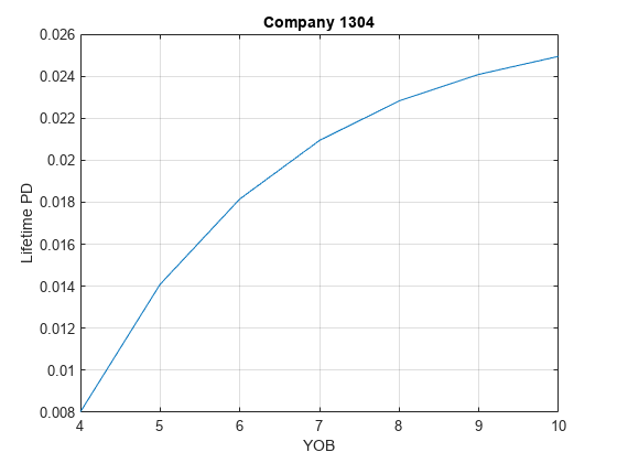
    1304    "Medium Risk"     4     2020    1.1     4.5       0.0080202 
    1304    "Medium Risk"     5     2021    0.9     1.5        0.014093 
    1304    "Medium Risk"     6     2022    1.2       5        0.018156 
    1304    "Medium Risk"     7     2023    1.4     5.5        0.020941 
    1304    "Medium Risk"     8     2024    1.6       6        0.022827 
    1304    "Medium Risk"     9     2025    1.8     6.5        0.024086 
    1304    "Medium Risk"    10     2026    1.8     6.5        0.024945 
    2067    "Low Risk"        7     2020    1.1     4.5       0.0015728 
    2067    "Low Risk"        8     2021    0.9     1.5       0.0027146 
    2067    "Low Risk"        9     2022    1.2       5        0.003431 
    2067    "Low Risk"       10     2023    1.4     5.5       0.0038939

Visualize the predicted lifetime PD for a company.

CompanyIDChoice = "1304";
CompanyID = str2double(CompanyIDChoice);
IndPlot = LifetimeData.ID==CompanyID;
plot(LifetimeData.YOB(IndPlot),LifetimeData.PredictedPD(IndPlot))
grid on
xlabel('YOB')
xticks(LifetimeData.YOB(IndPlot))
ylabel('Lifetime PD')
title(strcat("Company ",CompanyIDChoice))

Figure contains an axes object. The axes object with title Company 1304, xlabel YOB, ylabel Lifetime PD contains an object of type line.

Lifetime Prediction and Time Interval

Open Live Script

This example shows how time interval plays an important role for lifetime prediction when using a Logistic, Probit, or Cox model for probability of default (PD). Each PD value is a probability of default for the given "time interval" (for example, a time interval of 1 year), The data rows passed in for lifetime prediction must have the same periodicity as the time interval (that is, you can't pass a row that represents a quarter, and then a row that represents a year, and then one that represents 5 years. You must pass data for periods 1, 2, 3, 4,..., but not 1, 3, 7, 10, 20. Or if the time interval is 3, you must pass periods 3, 6, 9,... or 2, 5, 8,..., but not 3, 7, 15, 30.

Fit and Validate Model

load RetailCreditPanelData.mat
data = join(data,dataMacro);
head(data)

    ID    ScoreGroup    YOB    Default    Year     GDP     Market
    __    __________    ___    _______    ____    _____    ______

    1      Low Risk      1        0       1997     2.72      7.61
    1      Low Risk      2        0       1998     3.57     26.24
    1      Low Risk      3        0       1999     2.86      18.1
    1      Low Risk      4        0       2000     2.43      3.19
    1      Low Risk      5        0       2001     1.26    -10.51
    1      Low Risk      6        0       2002    -0.59    -22.95
    1      Low Risk      7        0       2003     0.63      2.78
    1      Low Risk      8        0       2004     1.85      9.48

Select a model type. The behavior of the data validation in predictLifetime depends on the model type. For more information, see Validation of Data Input for Lifetime Prediction.

The time interval in this example is 1. This value is stored in Cox models as the TimeInterval property and it is used for fitting and prediction.Logistic and Probit models do not store the time interval information.

ModelType = "cox";

pdModel = fitLifetimePDModel(data,ModelType,...
   'IDVar','ID','AgeVar','YOB',...
   'LoanVars','ScoreGroup','MacroVars',{'GDP' 'Market'},...
   'ResponseVar','Default');
disp(pdModel)

  Cox with properties:

           TimeInterval: 1
    ExtrapolationFactor: 1
                ModelID: "Cox"
            Description: ""
        UnderlyingModel: [1x1 CoxModel]
                  IDVar: "ID"
                 AgeVar: "YOB"
               LoanVars: "ScoreGroup"
              MacroVars: ["GDP"    "Market"]
            ResponseVar: "Default"

Conditional PD and Model Validation

The conditional PD values returned by predict are consistent with the time interval used for training the model. In this example, all PD values returned by predict are 1-year probabilities of default. There is no validation of the periodicity in the data input for predict.

dataPredictExample = data([1 2 6 10 15],:);
pdExample = predict(pdModel,dataPredictExample)

pdExample = 5×1

    0.0089
    0.0052
    0.0038
    0.0094
    0.0031

Model validation is done using the conditional PD returned by predict. Therefore, there is no row periodicity validation in modelDiscrimination or modelCalibration. However, model validation requires observed values of the response variable, and the definition of default used for the validation response values must be consistent with the training data. In other words, if the training data uses a time interval of 1, the validation response data cannot be defined with quarterly default data. There are no row-periodicity checks for modelDiscrimination or modelCalibration, it is assumed that the default definition in the validation data is consistent with the training data.

modelCalibrationPlot(pdModel,data,{'YOB','ScoreGroup'})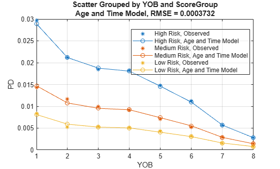

Figure contains an axes object. The axes object with title Scatter Grouped by YOB and ScoreGroup Cox, RMSE = 0.0003732, xlabel YOB, ylabel PD contains 6 objects of type line. One or more of the lines displays its values using only markers These objects represent High Risk, Observed, Medium Risk, Observed, Low Risk, Observed, High Risk, Cox, Medium Risk, Cox, Low Risk, Cox.

Lifetime PD

The predictLifetime function is used to compute lifetime PD. When making lifetime predictions:

A different data set is likely used, not the data you used for training and validation, but a new data set with forward-looking projections for different loans.
The projected values in the lifetime prediction data set span several periods ahead, potentially several years ahead.

Load the DataPredictLifetime.mat data for lifetime prediction. Note that for prediction, you don't need to pass the response data, you only pass predictors. You only pass response values for fitting or validation, not for prediction.

load DataPredictLifetime.mat
LifetimeData = join(LoanData,MacroScenario);
disp(LifetimeData)

     ID      ScoreGroup      YOB    Year    GDP    Market
    ____    _____________    ___    ____    ___    ______

    1304    "Medium Risk"     4     2020    1.1     4.5  
    1304    "Medium Risk"     5     2021    0.9     1.5  
    1304    "Medium Risk"     6     2022    1.2       5  
    1304    "Medium Risk"     7     2023    1.4     5.5  
    1304    "Medium Risk"     8     2024    1.6       6  
    1304    "Medium Risk"     9     2025    1.8     6.5  
    1304    "Medium Risk"    10     2026    1.8     6.5  
    2067    "Low Risk"        7     2020    1.1     4.5  
    2067    "Low Risk"        8     2021    0.9     1.5  
    2067    "Low Risk"        9     2022    1.2       5  
    2067    "Low Risk"       10     2023    1.4     5.5

The rows have yearly data, consistent with the time interval used for training. You can see this in both the Year variable and the YOB variable. There are no flags in this data set for lifetime predictions.

LifetimeData.PD = predict(pdModel,LifetimeData);
LifetimeData.LifetimePD = predictLifetime(pdModel,LifetimeData)

LifetimeData=11×8 table
     ID      ScoreGroup      YOB    Year    GDP    Market        PD        LifetimePD
    ____    _____________    ___    ____    ___    ______    __________    __________

    1304    "Medium Risk"     4     2020    1.1     4.5       0.0081336    0.0081336 
    1304    "Medium Risk"     5     2021    0.9     1.5       0.0063861     0.014468 
    1304    "Medium Risk"     6     2022    1.2       5       0.0047416     0.019141 
    1304    "Medium Risk"     7     2023    1.4     5.5       0.0028262     0.021913 
    1304    "Medium Risk"     8     2024    1.6       6       0.0014844     0.023365 
    1304    "Medium Risk"     9     2025    1.8     6.5       0.0014517     0.024783 
    1304    "Medium Risk"    10     2026    1.8     6.5       0.0014517     0.026198 
    2067    "Low Risk"        7     2020    1.1     4.5       0.0016091    0.0016091 
    2067    "Low Risk"        8     2021    0.9     1.5       0.0009006    0.0025082 
    2067    "Low Risk"        9     2022    1.2       5      0.00085273    0.0033588 
    2067    "Low Risk"       10     2023    1.4     5.5      0.00083391    0.0041899

When the periodicity of the rows does not match the periodicity in the training data, the lifetime PD values cannot be correctly computed.

Modify the selected rows using the SelectedRows variable in the code to see the behavior of predictLifetime as the periodicity of the data changes. (Alternatively, the YOB values can be manually modified to enter age increments inconsistent with the time interval of 1 year.)

RowSelection = "All rows";
switch RowSelection
   case "All rows"
      SelectedRows = 1:11; % Selecting all rows 1:11 is the same as the output above, no warnings
   case "Every other row"
      SelectedRows = 1:2:11; % Regular age increments, but skipping one year
   case "Irregular"
      SelectedRows = [1 2 7 8 11]; % Irregular age increments
end
LifetimeData2 = LifetimeData(SelectedRows,{'ID','ScoreGroup','YOB','Year','GDP','Market'});
disp(LifetimeData2)

     ID      ScoreGroup      YOB    Year    GDP    Market
    ____    _____________    ___    ____    ___    ______

    1304    "Medium Risk"     4     2020    1.1     4.5  
    1304    "Medium Risk"     5     2021    0.9     1.5  
    1304    "Medium Risk"     6     2022    1.2       5  
    1304    "Medium Risk"     7     2023    1.4     5.5  
    1304    "Medium Risk"     8     2024    1.6       6  
    1304    "Medium Risk"     9     2025    1.8     6.5  
    1304    "Medium Risk"    10     2026    1.8     6.5  
    2067    "Low Risk"        7     2020    1.1     4.5  
    2067    "Low Risk"        8     2021    0.9     1.5  
    2067    "Low Risk"        9     2022    1.2       5  
    2067    "Low Risk"       10     2023    1.4     5.5

LifetimeData2.PD = predict(pdModel,LifetimeData2);
LifetimeData2.LifetimePD = predictLifetime(pdModel,LifetimeData2);
disp(LifetimeData2)

     ID      ScoreGroup      YOB    Year    GDP    Market        PD        LifetimePD
    ____    _____________    ___    ____    ___    ______    __________    __________

    1304    "Medium Risk"     4     2020    1.1     4.5       0.0081336    0.0081336 
    1304    "Medium Risk"     5     2021    0.9     1.5       0.0063861     0.014468 
    1304    "Medium Risk"     6     2022    1.2       5       0.0047416     0.019141 
    1304    "Medium Risk"     7     2023    1.4     5.5       0.0028262     0.021913 
    1304    "Medium Risk"     8     2024    1.6       6       0.0014844     0.023365 
    1304    "Medium Risk"     9     2025    1.8     6.5       0.0014517     0.024783 
    1304    "Medium Risk"    10     2026    1.8     6.5       0.0014517     0.026198 
    2067    "Low Risk"        7     2020    1.1     4.5       0.0016091    0.0016091 
    2067    "Low Risk"        8     2021    0.9     1.5       0.0009006    0.0025082 
    2067    "Low Risk"        9     2022    1.2       5      0.00085273    0.0033588 
    2067    "Low Risk"       10     2023    1.4     5.5      0.00083391    0.0041899

The differences in behavior depend on the model type and whether the age variable is part of the model. You can change the model type in the fitting step to see the behavior for different model types. Remove the age variable (AgeVar) for Logistic and Probit models to observe the behavior when an age input argument is not part of the model. Note that an age input (AgeVar) argument is required for a Cox model. For more information, see Time Interval and Data Input for Lifetime Prediction.

Input Arguments

collapse all

`pdModel` — Probability of default model
`Logistic` object | `Probit` object | `Cox` object | `customLifetimePDModel` object

Probability of default model, specified as a previously created Logistic, Probit, or Cox object using fitLifetimePDModel. Alternatively, you can create a custom probability of default model using customLifetimePDModel.

Data Types: object

`data` — Lifetime data
table

Lifetime data, specified as a NumRows-by-NumCols table with projected predictor values to make lifetime predictions. The predictor names and data types must be consistent with the underlying model. The IDVar property of the pdModel input is used to identify the column containing the ID values in the table, and the IDs are used to identify rows corresponding to the different IDs and to make lifetime predictions for each ID.

Note

Rows passed in data for lifetime prediction must have the same periodicity as the time interval used to fit the model. For example, if the time interval used for training was one year, the data input for lifetime prediction cannot have quarterly data, or data for every five years.
Consecutive rows for the same ID must correspond to consecutive periods. For example, if the time interval used for training was one year, you cannot skip years and pass data for years 1, 2, 5, and 10.

For more information, see Data Input for Lifetime Prediction and Time Interval and Data Input for Lifetime Prediction.

Data Types: table

Name-Value Arguments

Specify optional pairs of arguments as Name1=Value1,...,NameN=ValueN, where Name is the argument name and Value is the corresponding value. Name-value arguments must appear after other arguments, but the order of the pairs does not matter.

Before R2021a, use commas to separate each name and value, and enclose Name in quotes.

Example: LifetimeData = predictLifetime(pdModel,Data,'ProbabilityType','survival')

`ProbabilityType` — Probability type
`'cumulative'` (default) | character vector with value `'cumulative'`, `'marginal'`, or `'survival'` | string with value `"cumulative"`, `"marginal"`, or `"survival"`

Probability type, specified as the comma-separated pair consisting of 'ProbabilityType' and a character vector or string.

Data Types: char | string

Output Arguments

collapse all

`LifeTimePredictedPD` — Predicted lifetime PD values
vector

Predicted lifetime PD values, returned as a NumRows-by-1 numeric vector.

More About

collapse all

Lifetime PD

Lifetime PD is the probability of a default event over the lifetime of a financial asset.

Lifetime PD typically refers to the cumulative default probability, given by

$P D_{c u m u l a t i v e} (t) = P {T \leq t}$

where T is the time to default.

For example, the predicted lifetime, cumulative PD for the second year is the probability that the borrower defaults any time between now and two years from now.

A closely related concept used for the computation of the lifetime Expected Credit Loss (ECL) is the marginal PD, given by

$P D_{m a r g i n a l} = P D_{c u m u l a t i v e} (t) - P D_{c u m u l a t i v e} (t - 1)$

A closely related probability is the survival probability, which is the complement of the cumulative probability and is reported as

$S (t) = P {T > t} = 1 - P D_{c u m u l a t i v e} (t)$

The following recursive formula shows the relationship between the conditional PDs and the survival probability:

$\begin{array}{l} S (t_{0}) = 1 \\ S (t_{1}) = S (t_{0}) (1 - P D (t_{1})) \\ ... \\ S (t_{n}) = S (t_{n - 1}) (1 - P D (t_{n})) \end{array}$

Where t_i - t_i-1 = Δt for all i = 1,...,n, and Δt is the time interval used to fit the model. For more information, see Time Interval for Logistic Models and Time Interval for Probit Models. In other words, because the PD values on the right-hand side of the formulas are probabilities of default for a period of length Δt, the increments between consecutive times in the recursion must always be of length Δt for all periods i = 1, 2,..., n.

The predictLifetime function calls the predict function to get the conditional PD and then converts it to survival, marginal, or lifetime cumulative PD using the previous formulas.

Data Input for Lifetime Prediction

Lifetime PD is the cumulative probability of default over multiple periods.

The input for the predictLifetime function should contain multiple rows per ID, where rows represent sequential time periods regularly spaced. In other words, the data should be in panel data form. The time interval between adjacent rows must be consistent with the time interval used to define the default binary variable in the training data. For more information, see Time Interval and Data Input for Lifetime Prediction.

If a dataset with one row per ID is passed, the output of predictLifetime is the same as the output of predict because the PD is predicted for one period only (see formulas in predict section). A dataset with multiple rows per ID allows predictLifetime to aggregate the default probability over multiple periods to get the cumulative PD.

The predictLifetime function is typically used for predictions on outstanding loans, where the predictor variable values must be projected, period by period, for several periods into the future. Although historical (training or testing) data sets in panel data form can be passed to predictLifetime, the typical workflow requires data preparation. It starts out with outstanding loans, where only the most recent values of the predictor variables are known. The data preparation then projects the predictor variable values into the future for multiple time periods, typically until the maturity of the loan for a lifetime analysis. For example, see Create Custom Lifetime PD Model for Decision Tree Model with Function Handle.

Time Interval and Data Input for Lifetime Prediction

The time interval used for fitting the model plays an important role for lifetime prediction.

The data input for predictLifetime is in panel data form, with multiple rows for each ID. There is an implicit or explicit time stamp for each row, and the time increments between consecutive rows must be the same as the time interval used to fit the model. For more information on time intervals, see Time Interval for Cox Models, Time Interval for Logistic Models, and Time Interval for Probit Models.

Following the notation of the lifetime PD recursive formulas described in Lifetime PD, the time stamps t₁, t₂,...,t_n between consecutive rows must satisfy t_i - t_i-1 = Δt for all i = 1,...,n, where Δt is the time interval used to fit the model. In other words:

Rows passed in the data input for lifetime prediction must have the same periodicity as the time interval used to fit the model. For example, if the time interval used for training was 1 year, the data input for lifetime prediction cannot have quarterly data, or data for every 5 years.
consecutive rows for the same ID must correspond to consecutive periods. For example, if the time interval used for training was 1 year, you cannot skip years and pass data for years 1, 2, 5, and 10.

Suppose, for concreteness, that the time interval Δt used to fit the model is 1 year. Then the PD values on the right-hand side of the formulas in Lifetime PD are 1-year PDs. Therefore:

Lifetime PD for quarterly data cannot be computed because S(1.25) ≄ S(1)(1 - PD(1.25)), since PD(1.25) is a 1-year PD spanning the default over the interval going from 0.25 to 1.25.
Lifetime PD for data every 5 years cannot be computed because S(10) ≄ S(5)(1 - PD(10)), since PD(10) is a 1-year PD spanning the default over the interval going from 9 to 10.
Lifetime PD for non-consecutive rows cannot be computed. For example, if the data input has rows corresponding to years 1, 2, 5 and 10, then S(1) and S(2) can be computed correctly, however S(5) ≄ S(2)(1-PD(5)) because PD(5) is a 1-year PD spanning the default over the interval going from 4 to 5, and similarly for S(10).

Validation of Data Input for Lifetime Prediction

The validation of the row periodicity in the data input for predictLifetime depends on the model type (ModelType) and whether the model contains an age variable (AgeVar).

Cox models can validate the periodicity of the data because the age variable (AgeVar) is a required input argument and Cox models store the time interval (TimeInterval) used to fit the model. The TimeInterval is used both to fit the model and to predict PD values. For more information on time intervals for a Cox model, see Time Interval for Cox Models. The age variable (AgeVar) is used as the time dimension. For each ID, if the periodicity of the data input, measured by the increments in the age variable, does not match the time interval used to train the model, a warning is displayed and the lifetime PD values are filled with NaNs.

Logistic and Probit models do not store the time interval value. However the predicted PD values are still consistent with the (explicit or implicit) time interval in the training data. For more information, see Time Interval for Logistic Models and Time Interval for Probit Models. Moreover, for Logistic and Probit models, the age variable (AgeVar) is optional, and there is no other way to specify a time dimension in the model. Therefore:

If the Logistic or Probit model has no age variable information, there is no way to validate the periodicity of the data. The lifetime PD is computed using the recursion in Lifetime PD, assuming that the periodicity is correct. It is the responsibility of the caller to ensure that the periodicity of the data rows is consistent with the time interval in the training data.
If the Logistic or Probit model has an age variable (AgeVar), this is used as a time dimension. However, because the time interval used to train the data is unknown for Logistic and Probit models, these models can only validate that the age increments are regular as follows, but cannot compare against a reference time interval.
- For each ID, when the age shows irregular age increments, there is a warning and the lifetime PD values are set to NaNs.
- When the age increments are regular within each ID, but some IDs have different age increments than others, a warning is displayed, but it is unknown which ID has the wrong increments. The lifetime PD values are computed using the recursion in Lifetime PD for all IDs. It is the responsibility of the caller to ensure that the periodicity of the data rows for all IDs is consistent with the time interval in the training data.

For an example, see Lifetime Prediction and Time Interval.

References

[1] Baesens, Bart, Daniel Roesch, and Harald Scheule. Credit Risk Analytics: Measurement Techniques, Applications, and Examples in SAS. Wiley, 2016.

[2] Bellini, Tiziano. IFRS 9 and CECL Credit Risk Modelling and Validation: A Practical Guide with Examples Worked in R and SAS. San Diego, CA: Elsevier, 2019.

[3] Breeden, Joseph. Living with CECL: The Modeling Dictionary. Santa Fe, NM: Prescient Models LLC, 2018.

[4] Roesch, Daniel and Harald Scheule. Deep Credit Risk: Machine Learning with Python. Independently published, 2020.

Version History

Introduced in R2020b

expand all

R2022b: Support for `customLifetimePDModel` model

The pdModel input supports an option for a customLifetimePDModel model object that you can create using customLifetimePDModel.

predictLifetime

Syntax

Description

Examples

Use Probit Lifetime PD Model to Predict Lifetime PD

Lifetime Prediction and Time Interval

Input Arguments

`pdModel` — Probability of default model
`Logistic` object | `Probit` object | `Cox` object | `customLifetimePDModel` object

`data` — Lifetime data
table

Name-Value Arguments

`ProbabilityType` — Probability type
`'cumulative'` (default) | character vector with value `'cumulative'`, `'marginal'`, or `'survival'` | string with value `"cumulative"`, `"marginal"`, or `"survival"`

Output Arguments

`LifeTimePredictedPD` — Predicted lifetime PD values
vector

More About

Lifetime PD

Data Input for Lifetime Prediction

Time Interval and Data Input for Lifetime Prediction

Validation of Data Input for Lifetime Prediction

References

Version History

R2022b: Support for `customLifetimePDModel` model

See Also

Topics

predictLifetime

Syntax

Description

Examples

Use Probit Lifetime PD Model to Predict Lifetime PD

Lifetime Prediction and Time Interval

Input Arguments

pdModel — Probability of default model Logistic object | Probit object | Cox object | customLifetimePDModel object

data — Lifetime data table

Name-Value Arguments

ProbabilityType — Probability type 'cumulative' (default) | character vector with value 'cumulative', 'marginal', or 'survival' | string with value "cumulative", "marginal", or "survival"

Output Arguments

LifeTimePredictedPD — Predicted lifetime PD values vector

More About

Lifetime PD

Data Input for Lifetime Prediction

Time Interval and Data Input for Lifetime Prediction

Validation of Data Input for Lifetime Prediction

References

Version History

R2022b: Support for customLifetimePDModel model

See Also

Topics

`pdModel` — Probability of default model
`Logistic` object | `Probit` object | `Cox` object | `customLifetimePDModel` object

`data` — Lifetime data
table

`ProbabilityType` — Probability type
`'cumulative'` (default) | character vector with value `'cumulative'`, `'marginal'`, or `'survival'` | string with value `"cumulative"`, `"marginal"`, or `"survival"`

`LifeTimePredictedPD` — Predicted lifetime PD values
vector

R2022b: Support for `customLifetimePDModel` model