rfsystem
Generate RF Blockset model and perform circuit envelope or idealized baseband simulation
Description
Use the rfsystem
System object™ to generate RF Blockset™ model and perform circuit envelope and idealized
baseband (since R2023a) simulation of an RF system designed using an rfbudget object. This
object supports vector inputs and has no limitations on the frame size.
Note
You can add or delete RF Blockset blocks from the model but you cannot modify the parameters of the
Inport and Outport blocks. After this update, the input
rfbudget object to the rfsystem will be preserved and
you can inspect this rfbudget object using the RF Budget
Analyzer app.
To perform circuit envelope simulation of an RF system:
Create the
rfsystemobject and set its properties.Call the object with arguments, as if it were a function.
To learn more about how System objects work, see What Are System Objects?
Creation
Description
rfs = rfsystem(rfb)rfb and perform circuit
envelope or idealized baseband (since R2023a) simulation.
Use Object Functions to open, save, close, or hide the RF Blockset model.
rfs = rfsystem(rfb,Name=Value)rfsystem(rfb,'ModelName'='rfmodel') sets the
name of the RF Blockset model to rfmodel.
Properties
Usage
Syntax
Description
out = rfs(in)out using input signal values in. Pass
in as an input argument to an automatically-generated RF Blockset model.
You can design four architectures, RF to RF, DC to RF, RF to DC, and DC to DC, using
the rfsystem object. For more information, see Design RF-RF, IQ-RF, RF-IQ, and IQ-IQ Architectures.
Note
Passing multiple input vectors and concatenating the output vectors is equivalent to performing one long simulation with a vertically-concatenated input.
Input Arguments
Output Arguments
Object Functions
To use an object function, specify the
System object as the first input argument. For
example, to release system resources of a System object named obj, use
this syntax:
release(obj)
Examples
Design an RF receiver to perform circuit envelope simulation.
Create fifth- and seventh-order bandpass RF filters.
f1 = rffilter(ResponseType="Bandpass",FilterOrder=5, ...
        PassbandFrequency=[4.85 5.15]*1e9);
f2 = rffilter(ResponseType="Bandpass",FilterOrder=7, ...
        PassbandFrequency=[10 130]*1e6);
Create two amplifier objects with 3 dB and 5 dB gain, respectively.
a1 = amplifier(Gain=3,NF=1.53,OIP3=35);
a2 = amplifier(Gain=5,NF=8,OIP3=37);
Create a modulator with a local frequency of 4.93 GHz.
d = modulator(Gain=0,NF=4,OIP3=50,LO=4.93e9, ...
        ConverterType="Down");
Design an RF receiver with the budget elements at an input frequency of 5 GHz, an available input power of -30 dBm, and a bandwidth of 200 MHz.
rfb = rfbudget([f1 a1 d f2 a2],5e9,-30,200e6);
Create an RF system for the RF receiver using the rfbudget object.
rfs = rfsystem(rfb);
Specify input time-domain signal for the RF system.
in = [1e-3*ones(8,1); zeros(8,1)] .* ones(1,10);
in = in(:);
Calculate the output time-domain signal of the RF system.
out = rfs(in);
out = [out; rfs(in)];
Specify the sample time of the RF system.
t = rfs.SampleTime*(0:length(out)-1);
Plot the simulated output.
plot(t,[in; in],'-o',t,abs(out),'-+')
grid on

Release system resources and turn off fast restart.
release(rfs)
Open an RF Blockset model of the designed RF system using the open_system object function.
open_system(rfs)

Design four different chain architectures using an RF System object.
Create an input column vector.
in = (1:8)';
Design RF-RF Architecture
Create an rfbudget object using an amplifier object.
a = amplifier;
Calculate the RF budget of the amplifier at an input frequency of 5 GHz, an available input power of –30 dBm, and a bandwidth of 10 KHz.
rfb = rfbudget(a,5e9,-30,10e3);
Create an RF system using the rfbudget object.
rfs = rfsystem(rfb);
Create an RF-RF architecture using the input column vector.
out0 = rfs(in);
Release system resources and turn off fast restart.
release(rfs)
Open an RF Blockset model of the RF system.
open_system(rfs)

Design IQ-RF Architecture
Use a modulator object with an upconverter to create an rfbudget object.
u = modulator('ConverterType','Up','LO',1e9);
Calculate the RF budget of the modulator at an input frequency of 0 GHz, an available input power of –30 dBm, and a bandwidth of 10 KHz.
rfb2 = rfbudget(u,0,-30,10e3);
Create an RF system using the rfbudget object.
rfs2 = rfsystem(rfb2);
Create an IQ-RF architecture using the input column vector.
inI = in;
inQ = in;
out = rfs2(inI,inQ);
Release system resources and turn off fast restart.
release(rfs2)
Open an RF Blockset model of the RF system.
open_system(rfs2)

Design RF-IQ Architecture
Use a modulator object with a downconverter to create an rfbudget object.
d = modulator('ConverterType','Down','LO',1e9);
Calculate the RF budget of the modulator at an input frequency of 1 GHz, an available input power of –30 dBm, and a bandwidth of 10 KHz.
rfb3 = rfbudget(d,1e9,-30,10e3);
Create an RF system using the rfbudget object.
rfs3 = rfsystem(rfb3);
Create an RF-IQ architecture using the input column vector.
[outI,outQ] = rfs3(in);
Release system resources and turn off fast restart.
release(rfs3)
Open an RF Blockset model of the RF system.
open_system(rfs3)

Design IQ-IQ Architecture
Create an rfbudget object using an amplifier object.
a1 = amplifier;
Calculate the RF budget of the amplifier at an input frequency of 0 GHz, an available input power of –30 dBm, and a bandwidth of 10 KHz.
rfb4 = rfbudget(a1,0,-30,10e3);
Create an RF system using the rfbudget object.
rfs4 = rfsystem(rfb4);
Create an IQ-IQ architecture using the input column vector.
[outI2,outQ2] = rfs4(inI,inQ);
Release system resources and turn off fast restart.
release(rfs4)
Open an RF Blockset model of the RF system.
open_system(rfs4)

Create a fifth-order bandpass RF filter.
f1 = rffilter(ResponseType="Bandpass",FilterOrder=5, ...
   PassbandFrequency=[4.85 5.15]*1e9);
Create an amplifier with 3 dB gain.
a1 = amplifier(Gain=3,NF=1.53,OIP3=35);
Create a modulator with a local frequency of 4.93 GHz.
d = modulator(Gain=0,NF=4,OIP3=50,LO=4.93e9, ...
   ConverterType="Down");
Create a seventh-order bandpass RF filter.
f2 = rffilter(ResponseType="Bandpass",FilterOrder=7, ...
   PassbandFrequency=[10 130]*1e6);
Create another amplifier with a 3 dB gain.
a2 = amplifier(Gain=5,NF=8,OIP3=37);
Design an RF receiver with the budget elements at an input frequency of 5 GHz, an available input power of –30 dBm, and a bandwidth of 200 MHz.
b = rfbudget([f1 a1 d f2 a2],5e9,-30,200e6);
Duplicate the budget chain into a multiple-input single-output receiver (MISO) system with four branches.
rfs = rfsystem(b,Rx=4);
Open the underlying RF system model to inspect the MISO receiver
open_system(rfs)
![]()
set_param(bdroot,'ZoomFactor','FitSystem')
Create four inputs to the MISO receiver. The pulsed carrier square wave input is time-sliced into four pieces.
in1 = [1e-3*[1;1;0;0;0;0;0;0]; zeros(8,1)] .* ones(1,10);
in1 = in1(:);
in2 = [1e-3*[0;0;1;1;0;0;0;0]; zeros(8,1)] .* ones(1,10);
in2 = in2(:);
in3 = [1e-3*[0;0;0;0;1;1;0;0]; zeros(8,1)] .* ones(1,10);
in3 = in3(:);
in4 = [1e-3*[0;0;0;0;0;0;1;1]; zeros(8,1)] .* ones(1,10);
in4 = in4(:);
out = rfs(in1,in2,in3,in4);
Release system resources and turn off fast restart.
release(rfs)
reset(rfs)
Plot the circuit envelope simulated result.
t = rfs.SampleTime*(0:length(out)-1);
plot(t,in1+in2+in3+in4,'-o',t,abs(out),'-+')
grid on
![]()
Type rfBudgetAnalyzer(rfs) command at the command line to open the MISO receiver in the RF Budget Analyzer app to visualize the initial budget chain b.

Duplicate the budget chain into a single-input multiple-output (SIMO) array system with sixteen branches.
rfs2 = rfsystem(b,Tx=16);
Open the underlying RF system model to inspect the SIMO receiver
open_system(rfs2)
![]()
Type this command at the MATLAB® command line to create 16 outputs to the SIMO transmitter.
[out1(1:16).val] = rfs2(in1);
Create a fifth-order bandpass RF filter.
f1 = rffilter(ResponseType="Bandpass",FilterOrder=5,PassbandFrequency=[4.85 5.15]*1e9);
Create an amplifier with the gain of 3 dB, noise figure of 1.53 dB, and OIP3 of 35 dBm.
a1 = amplifier(Gain=3,NF=1.53,OIP3=35);
Create an rfbudget object using these elements at an input frequency of 5 GHz, an available input power of -30 dBm, and a bandwidth of 200 MHz.
rfb = rfbudget([f1 a1],5e9,-30,200e6);
Create an RF system using the rfbdget object. Name the model and save the RF Blockset model.
rfs = rfsystem(rfb,ModelName="myRFSystem_Model")
save_system(rfs);
rfs =

  rfsystem with properties:

          ModelName: 'myRFSystem_Model'
         SampleTime: 6.2500e-10
     InputFrequency: 5.0000e+09
    OutputFrequency: 5.0000e+09
           RFInputs: 1
          RFOutputs: 1
            Library: 'CircuitEnvelope'
Design an RF receiver using the rfsystem System object. View the object in the RF Budget Analyzer app to perform harmonic balance (HB) analysis.
Create fifth- and seventh-order bandpass RF filters.
f1 = rffilter(ResponseType="Bandpass",FilterOrder=5, ...
        PassbandFrequency=[4.85 5.15]*1e9);
f2 = rffilter(ResponseType="Bandpass",FilterOrder=7, ...
        PassbandFrequency=[10 130]*1e6);
Create two amplifier objects with 3 dB and 5 dB gain, respectively.
a1 = amplifier(Gain=3,NF=1.53,OIP3=35);
a2 = amplifier(Gain=5,NF=8,OIP3=37);
Create a modulator with a local frequency of 4.93 GHz.
d = modulator(Gain=0,NF=4,OIP3=50,LO=4.93e9, ...
        ConverterType="Down");
Design an RF receiver with the budget elements at an input frequency of 5 GHz, an available input power of – 30 dBm, and a bandwidth of 10 MHz.
rfb = rfbudget([f1 a1 d f2 a2],5e9,-30,10e6);
Create an RF system for the RF receiver using the rfbudget object.
rfs = rfsystem(rfb);
Open an RF Blockset model of the designed RF system using the open_system function.
open_system(rfs)

Type rfBudgetAnalyzer(rfs) command at the MATLAB® command line to open this RF system in the RF Budget Analyzer app.
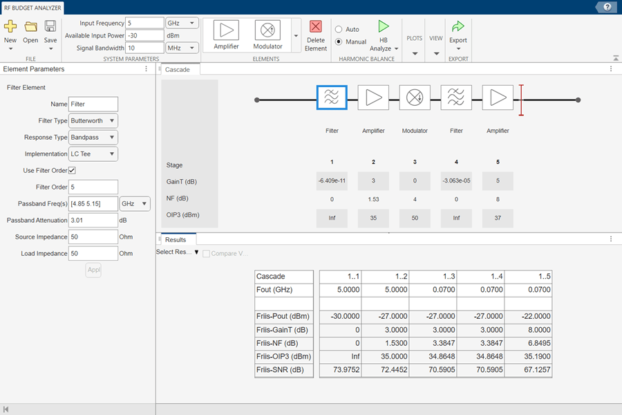
To conduct HB analysis in the app, click the HB-Analyze button.

Since R2025a
This example shows you how to account mismatch loss between two elements in an RF chain. To do this:
First, define system parameters and construct RF elements.
Second, create an
rfbudgetobject to construct an RF chain with the elements that you have designed in the first step and compute its RF budget.Finally, input this
rfbudgetobject to an RF System object™ to create an RF Blockset model and simulate to account mismatch loss between two elements.
You can choose to simulate your RF chain with either circuit envelope or idealized baseband simulation. This example compares:
Simulation fidelity between circuit envelope or idealized baseband simulation.
Simulated output with RF budget results.
Define System Parameters
Define input frequency, signal bandwidth, and input power.
fin = 4e9;
bw = 5e6;
in_dBm = -30;
Create RF Elements
Create an amplifier, n-port device, modulator, and RF filter.
a = amplifier( ...
    Gain = 31, ...
    Zin = 41+15i, ...
    Zout = 92+65i);
s = nport('passive.s2p');
m = modulator( ...
    LO = 1e9, ...
    Gain = 42, ...
    Zin = 35+89i, ...
    Zout = 79+32i);
r = rffilter( ...
    PassbandFrequency = fin+1e9-bw/2, ...
    Zin = 38, ...
    Zout = 38);
Create RF Budget and Construct RF Chain
Create rfbudget object and calculate its RF budget.
rfobj = rfbudget([a s m r],fin,in_dBm,bw);
Simulate RF Chain in Circuit Envelope Simulation Environment
Input this budget object to an rfsystem System object. The rfsystem object enables you to simulate your RF chain using circuit envelope and idealized baseband simulation.
Build your RF chain using circuit envelope simulation. Circuit envelope simulation allows multicarrier simulation of RF networks with arbitrary topology. It also allows impedance mismatches. Estimate the computation time using tic and toc functions.
tic
rfsCE = rfsystem(rfobj);
toc
Elapsed time is 64.615709 seconds.
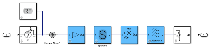
Open the system modeled using circuit envelope blocks in Simulink.
open_system(rfsCE)
To simulate, first load the MAT file containing the 5G NR baseband input signal.
load('input.mat');
input = input(1:400);
Turn off the noise so that you can compare circuit envelope and idealized baseband simulations.
set_param([rfsCE.ModelName '/Configuration1'],'AddNoise','off')
Define the input signal for rfsystem object.
tic
outCE = rfsCE(input);
tocCE = toc
tocCE =

   28.5573
Simulate RF Chain in Idealized Baseband Simulation Environment
Build your RF chain using idealized baseband simulation. Estimate the computation time using tic and toc functions. This allows you to analyze a cascade of mathematical models of RF components within the MATLAB® environment. The Idealized Baseband System objects assume perfect impedance matching. However, by using Mismatch property in rfsystem System object, you can account for mismatch loss between two elements in an RF chain in your simulation. Estimate the computation time using tic and toc functions.
tic
rfsIdeal = rfsystem(rfobj,'Library','IdealizedBaseband','Mismatch',true);
toc
Elapsed time is 9.478470 seconds.
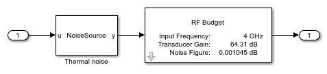
Open the system modeled using idealized baseband blocks in Simulink.
open_system(rfsIdeal)
Turn off the noise so that you can compare circuit envelope and idealized baseband simulations.
set_param([rfsIdeal.ModelName '/Thermal noise'],'NoiseSrc','None')
tic
outIdeal = rfsIdeal(input);
tocIdeal = toc
tocIdeal =

    5.0207
Plot Simulation Fidelity
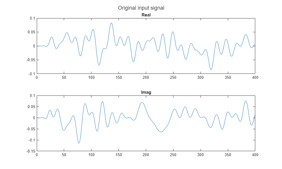
Plot the real and imaginary components of the original input signal.
f1 = figure;
subplot(2,1,1),plot(real(input)),title('Real')
subplot(2,1,2),plot(imag(input)),title('Imag')
sgtitle('Original input signal')
Compare circuit envelope and idealized baseband simulations and observe the simulation fidelity overlaps.
f2 = figure;
subplot(2,1,1),plot(real(outCE)),hold('on'),plot(real(outIdeal),'+')
legend(['CE - ' num2str(tocCE) ' seconds'],['Ideal - ' num2str(tocIdeal) ' seconds'])
title('Real')
subplot(2,1,2),plot(imag(outCE)),hold('on'),plot(imag(outIdeal),'+')
legend(['CE - ' num2str(tocCE) ' seconds'],['Ideal - ' num2str(tocIdeal) ' seconds'])
title('Imag')
sgtitle('Simulation fidelity between circuit envelope and idealized baseband simulation')
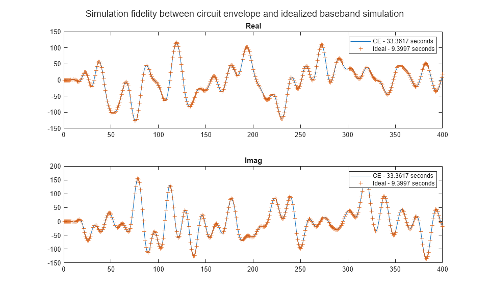
Observe the simulation fidelity between two solvers and their computation time. The data points overlap.
Compare Simulation Results to RF Budget Output
Release the rfsystem System object from fast restart.
release(rfsCE)
release(rfsIdeal)

Define the input signal to the system.
in_DC = 10^((in_dBm-30)/20)*((1+1j)/sqrt(2));
Observe that circuit envelope and idealized baseband simulations give similar output power.
outCE_DC = rfsCE(in_DC);
outIdeal_DC = rfsIdeal(in_DC);
outCE_DC_dBm = 20*log10(abs(outCE_DC)) + 30
outIdeal_DC_dBm = 20*log10(abs(outIdeal_DC)) + 30
outCE_DC_dBm =

   34.2893


outIdeal_DC_dBm =

   34.2893
Observe the output power computed from the rfbudget object.
Note that the mismatch loss calculations using the rfsystem and rfbudget objects are based on the computeBudget method, but output power calculations between these two objects differ because mismatch loss calculations employ rational interpolation to ensure causality and passivity for transient simulation, whereas rfbudget does not.
rfbudget_DC_dBm = rfobj.OutputPower(end)
rfbudget_DC_dBm =

   34.3116
Tips
Create multiple
rfsystemoutputs using this optional syntax:[
out(1:n).val] =rfs(in), where
nis the number of output chains in a single-input multiple-output (SIMO) transmitter system 'Tx' using the input signalin.