rlMDPEnv

Create Markov decision process environment for reinforcement learning

Description

A Markov decision process (MDP) is a discrete-time stochastic control process in which the state and observation belong to finite spaces, and stochastic rules govern state transitions. It provides a mathematical framework for modeling decision making in situations where outcomes are partly random and partly under the control of the decision maker. MDPs are useful for studying optimization problems solved using reinforcement learning. Use rlMDPEnv to create a Markov decision process environment for reinforcement learning in MATLAB^®.

Creation

Syntax

env = rlMDPEnv(MDP)

Description

env = rlMDPEnv(MDP) creates a reinforcement learning environment env with the specified MDP model.

Input Arguments

MDP — Markov decision process model

GridWorld object | GenericMDP object

Markov decision process model, specified as one of these objects:

• GridWorld object created using the createGridWorld function

• GenericMDP object created using the createMDP function

Properties

Model — Markov decision process model

GridWorld object | GenericMDP object

Markov decision process model, specified as a GridWorld object or GenericMDP object.

Example: env.Model=createMDP(3,["left";"right"])

ResetFcn — Reset function

function handle

Reset function, specified as a function handle.

Example: env.ResetFcn=@() randi(3)

Object Functions

getActionInfo	Obtain action data specifications from reinforcement learning environment, agent, or experience buffer
getObservationInfo	Obtain observation data specifications from reinforcement learning environment, agent, or experience buffer
sim	Simulate trained reinforcement learning agents within specified environment
train	Train reinforcement learning agents within a specified environment
validateEnvironment	Validate custom reinforcement learning environment

Examples

Create Grid World Environment

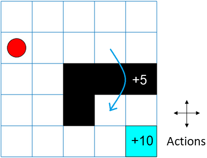
For this example, create a 5-by-5 grid world object with these rules:

1. A 5-by-5 grid world bounded by borders, with four possible actions: North = 1, South = 2, East = 3, West = 4.

2. The agent begins from cell [2,1] (second row, first column, indicated by the red circle in the figure).

3. The agent receives reward +10 if it reaches the terminal state at cell [5,5] (blue cell).

4. The environment contains a special jump from cell [2,4] to cell [4,4] with +5 reward (blue arrow).

5. The agent is blocked by obstacles in cells [3,3], [3,4], [3,5], and [4,3] (black cells).

6. All other actions result in –1 reward.

Then, use the gridworld object to create an environment for which you can train and simulate an agent.

First, create a GridWorld object using the createGridWorld function.

gw = createGridWorld(5,5)

gw = 
  GridWorld with properties:

                GridSize: [5 5]
            CurrentState: "[1,1]"
                  States: [25×1 string]
                 Actions: [4×1 string]
                       T: [25×25×4 double]
                       R: [25×25×4 double]
          ObstacleStates: [0×1 string]
          TerminalStates: [0×1 string]
    ProbabilityTolerance: 8.8818e-16

Display the action names.

gw.Actions

ans = 4×1 string
    "N"
    "S"
    "E"
    "W"

Then set the initial, terminal, and obstacle states.

gw.CurrentState = "[2,1]";
gw.TerminalStates = "[5,5]";
gw.ObstacleStates = ["[3,3]";"[3,4]";"[3,5]";"[4,3]"];

Update the state transition matrix for the obstacle states.

updateStateTranstionForObstacles(gw)

To set the jump rule over the obstacle states, first zero out all the transitions out from state "[2,4]" for any action. Note that, because each number in one row represents a probability of moving into a specific cell, all the numbers along a row must always add to either one or zero, otherwise an error is thrown.

Set to zero the probability of transitioning out from state "[2,4]". Use the state2idx function to obtain the index associated with the state "[2,4]".

gw.T(state2idx(gw,"[2,4]"),:,:) = 0;

Then, for any action, set to one the probability from transitioning from state "[2,4]" to state "[4,4]".

gw.T(state2idx(gw,"[2,4]"),state2idx(gw,"[4,4]"),:) = 1;

Next, define the rewards in the reward transition matrix.

nS = numel(gw.States);
nA = numel(gw.Actions);
gw.R = -1*ones(nS,nS,nA);
gw.R(state2idx(gw,"[2,4]"),state2idx(gw,"[4,4]"),:) = 5;
gw.R(:,state2idx(gw,gw.TerminalStates),:) = 10;

Use rlMDPEnv to create the grid world environment env from the GridWorld object gw.

env = rlMDPEnv(gw)

env = 
  rlMDPEnv with properties:

       Model: [1×1 rl.env.GridWorld]
    ResetFcn: []

You can visualize the grid world environment using the plot function.

plot(env)

Use the action2idx function to obtain the index associated with the "E" action. Then use the environment step function to move the agent eastward.

[xn,rn,id]=step(env,action2idx(env.Model,"E"))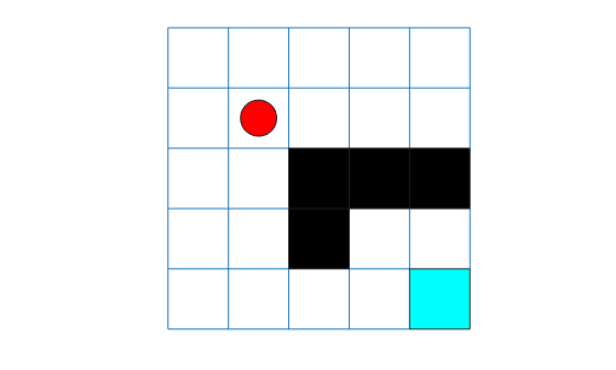

xn = 
7

rn = 
-1

id = logical
   0

Use the idx2state function to display the name of the next state.

idx2state(env.Model,xn)

ans = 
"[2,2]"

Use the getActionInfo and getObservationInfo functions to extract the action and observation specification objects from the environment.

actInfo = getActionInfo(env)

actInfo = 
  rlFiniteSetSpec with properties:

       Elements: [4×1 double]
           Name: "MDP Actions"
    Description: [0×0 string]
      Dimension: [1 1]
       DataType: "double"

obsInfo = getObservationInfo(env)

obsInfo = 
  rlFiniteSetSpec with properties:

       Elements: [25×1 double]
           Name: "MDP Observations"
    Description: [0×0 string]
      Dimension: [1 1]
       DataType: "double"

You can now use the action and observation specifications to create an agent for env, and then use the train and sim functions to train and simulate the agent within the environment.

Version History

Introduced in R2019a