interpolateTemperature
Interpolate temperature in thermal result at arbitrary spatial locations
Syntax
Description
Tintrp = interpolateTemperature(thermalresults,xq,yq)xq and yq for a steady-state thermal
model.
Tintrp = interpolateTemperature(thermalresults,querypoints)querypoints for a steady-state thermal model.
Examples
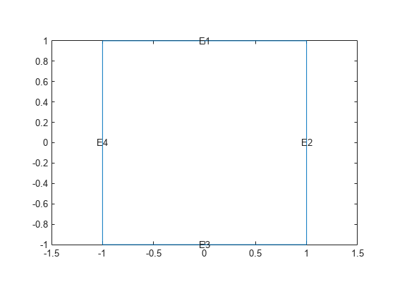
Create and plot a square geometry.
R1 = [3,4,-1,1,1,-1,1,1,-1,-1]';
g = decsg(R1, 'R1', ('R1')');
pdegplot(g,EdgeLabels="on")
xlim([-1.1,1.1])
ylim([-1.1,1.1])
Create an femodel object for steady-state thermal analysis and include the geometry into the model.
model = femodel(AnalysisType="thermalSteady", ...
                Geometry=g);
Assuming that this is an iron plate, assign a thermal conductivity of 79.5 W/(m*K). For steady-state analysis, you do not need to assign mass density or specific heat values.
model.MaterialProperties = ...
    materialProperties(ThermalConductivity=79.5);
Apply a constant temperature of 300 K to the bottom of the plate (edge 3).
model.EdgeBC(3) = edgeBC(Temperature=300);
Apply convection on the two sides of the plate (edges 2 and 4).
model.EdgeLoad([2 4]) = ...
    edgeLoad(ConvectionCoefficient=25,...
             AmbientTemperature=50);
Mesh the geometry and solve the problem.
model = generateMesh(model);
R = solve(model)
R =
  SteadyStateThermalResults with properties:

    Temperature: [1529×1 double]
     XGradients: [1529×1 double]
     YGradients: [1529×1 double]
     ZGradients: []
           Mesh: [1×1 FEMesh]
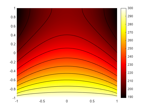
The solver finds the values of temperatures and temperature gradients at the nodal locations. To access these values, use R.Temperature, R.XGradients, and so on. For example, plot the temperatures at nodal locations.
figure;
pdeplot(R.Mesh,XYData=R.Temperature,...
        Contour="on",ColorMap="hot");
axis equal
Interpolate the resulting temperatures to a grid covering the central portion of the geometry, for x and y from -0.5 to 0.5.
v = linspace(-0.5,0.5,11);
[X,Y] = meshgrid(v);

Tintrp = interpolateTemperature(R,X,Y);
Reshape the Tintrp vector and plot the resulting temperatures.
Tintrp = reshape(Tintrp,size(X));

figure
contourf(X,Y,Tintrp)
colormap(hot)
colorbar
axis equal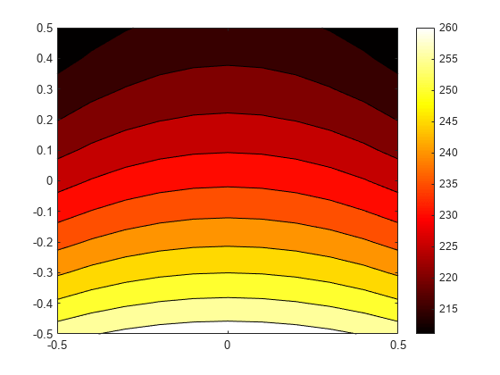
Alternatively, you can specify the grid by using a matrix of query points.
querypoints = [X(:),Y(:)]';
Tintrp = interpolateTemperature(R,querypoints);
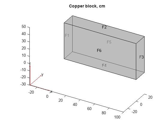
Create an femodel object for steady-state thermal analysis and include a block geometry into the model.
model = femodel(AnalysisType="thermalSteady", ...
                Geometry="Block.stl");
Plot the geometry.
pdegplot(model.Geometry,FaceLabels="on",FaceAlpha=0.5)
title("Copper block, cm")
Assuming that this is a copper block, the thermal conductivity of the block is approximately 4 W/(cm*K).
model.MaterialProperties = ...
    materialProperties(ThermalConductivity=4);
Apply a constant temperature of 373 K to the left side of the block (edge 1) and a constant temperature of 573 K at the right side of the block.
model.FaceBC(1) = faceBC(Temperature=373);
model.FaceBC(3) = faceBC(Temperature=573);
Apply a heat flux boundary condition to the bottom of the block.
model.FaceLoad(4) = faceLoad(Heat=-20);
Mesh the geometry and solve the problem.
model = generateMesh(model);
R = solve(model)
R =
  SteadyStateThermalResults with properties:

    Temperature: [12822×1 double]
     XGradients: [12822×1 double]
     YGradients: [12822×1 double]
     ZGradients: [12822×1 double]
           Mesh: [1×1 FEMesh]
The solver finds the values of temperatures and temperature gradients at the nodal locations. To access these values, use results.Temperature, results.XGradients, and so on. For example, plot temperatures at nodal locations.
pdeplot3D(R.Mesh,ColorMapData=R.Temperature)
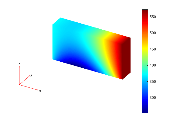
Create a grid specified by x, y, and z coordinates and interpolate temperatures to the grid.
[X,Y,Z] = meshgrid(1:16:100,1:6:20,1:7:50);

Tintrp = interpolateTemperature(R,X,Y,Z);
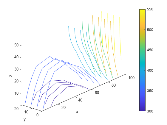
Create a contour slice plot for fixed values of the y coordinate.
Tintrp = reshape(Tintrp,size(X));
figure
contourslice(X,Y,Z,Tintrp,[],1:6:20,[])
xlabel("x")
ylabel("y")
zlabel("z")
xlim([1,100])
ylim([1,20])
zlim([1,50])
axis equal
view(-50,22)
colorbar
Alternatively, you can specify the grid by using a matrix of query points.
querypoints = [X(:),Y(:),Z(:)]';
Tintrp = interpolateTemperature(R,querypoints);
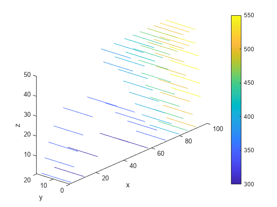
Create a contour slice plot for four fixed values of the z coordinate.
Tintrp = reshape(Tintrp,size(X));
figure
contourslice(X,Y,Z,Tintrp,[],[],1:7:50)
xlabel("x")
ylabel("y")
zlabel("z")
xlim([1,100])
ylim([1,20])
zlim([1,50])
axis equal
view(-50,22)
colorbar
Solve a 2-D transient heat transfer problem on a square domain and compute temperatures at the convective boundary.
Create and plot a square geometry.
g = @squareg;
pdegplot(g,EdgeLabels="on")
xlim([-1.1,1.1])
ylim([-1.1,1.1])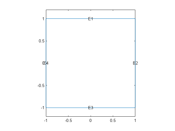
Create an femodel object for transient thermal analysis and include the geometry into the model.
model = femodel(AnalysisType="thermalTransient", ...
                Geometry=g);
Assign the following thermal properties:
Thermal conductivity is 100 W/(m*C)
Mass density is 7800 kg/m^3
Specific heat is 500 J/(kg*C)
model.MaterialProperties = ...
    materialProperties(ThermalConductivity=100,...
                       MassDensity=7800,...
                       SpecificHeat=500);
Apply a convection boundary condition on the right edge.
model.EdgeLoad(2) = ...
    edgeLoad(ConvectionCoefficient=5000,...
             AmbientTemperature=25);
Set the initial conditions: uniform room temperature across domain and higher temperature on the left edge.
model.FaceIC = faceIC(Temperature=25);
model.EdgeIC(4) = edgeIC(Temperature=100);
Generate a mesh and solve the problem using 0:1000:200000 as a vector of times.
model = generateMesh(model);
tlist = 0:1000:200000;
R = solve(model,tlist);
Define a line at convection boundary and compute temperature gradients across that line.
X = -1:0.1:1;
Y = ones(size(X));
Tintrp = interpolateTemperature(R,X,Y,1:length(tlist));
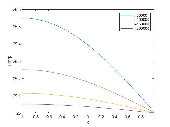
Plot the interpolated temperature Tintrp along the x axis for the following values from the time interval tlist.
figure
t = 51:50:201;
p = gobjects(size(t));
for i = 1:numel(t)
  p(i) = plot(X,Tintrp(:,t(i)), ...
      DisplayName="T="+tlist(t(i)));
  hold on
end
legend(p)
xlabel("x")
ylabel("Tintrp")
Input Arguments
Output Arguments
Version History
Introduced in R2017a