evaluateHeatFlux
Evaluate heat flux of thermal solution at nodal or arbitrary spatial locations
Syntax
Description
[ returns the heat
flux for a 2-D problem at the nodal points of the triangular mesh.qx,qy]
= evaluateHeatFlux(thermalresults)
[ returns the heat
flux for a 3-D thermal problem at the nodal points of the tetrahedral
mesh.qx,qy,qz]
= evaluateHeatFlux(thermalresults)
[
returns the heat flux for a thermal problem at the 2-D points specified in
qx,qy]
= evaluateHeatFlux(thermalresults,xq,yq)xq and yq. This syntax is valid for
both the steady-state and transient thermal models.
[___] = evaluateHeatFlux(
returns the heat flux for a thermal problem at the 2-D or 3-D points specified
in thermalresults,querypoints)querypoints. This syntax is valid for both the
steady-state and transient thermal models.
[___] = evaluateHeatFlux(___,
returns the heat flux for a thermal problem at the times specified in
iT)iT. You can specify iT after the
input arguments in any of the previous syntaxes.
The first dimension of qx, qy, and,
in the 3-D case, qz represents the node indices or
corresponds to query points. The second dimension corresponds to time steps
iT.
Examples
For a 2-D steady-state thermal problem, evaluate heat flux at the nodal locations and at the points specified by x and y coordinates.
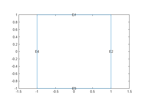
Create and plot a unit square geometry.
R1 = [3,4,-1,1,1,-1,1,1,-1,-1]';
g = decsg(R1,'R1',('R1')');
pdegplot(g,EdgeLabels="on")
xlim([-1.1 1.1])
ylim([-1.1 1.1])
Create an femodel object for steady-state thermal analysis and include the geometry into the model.
model = femodel(AnalysisType="thermalSteady", ...
                Geometry=g);
Assuming that this geometry represents an iron plate, the thermal conductivity is .
model.MaterialProperties = ...
    materialProperties(ThermalConductivity=79.5);
Apply a constant temperature of 500 K to the bottom of the plate (edge 3).
model.EdgeBC(3) = edgeBC(Temperature=500);
Apply convection on the two sides of the plate (edges 2 and 4).
model.EdgeLoad([2 4]) = ...
    edgeLoad(ConvectionCoefficient=25,...
             AmbientTemperature=50);
Mesh the geometry and solve the problem.
model = generateMesh(model);
R = solve(model)
R =
  SteadyStateThermalResults with properties:

    Temperature: [1529×1 double]
     XGradients: [1529×1 double]
     YGradients: [1529×1 double]
     ZGradients: []
           Mesh: [1×1 FEMesh]
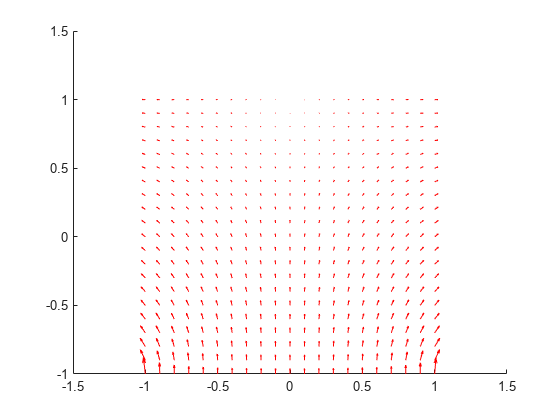
Evaluate heat flux at the nodal locations.
[qx,qy] = evaluateHeatFlux(R);
figure
pdeplot(R.Mesh,FlowData=[qx qy])
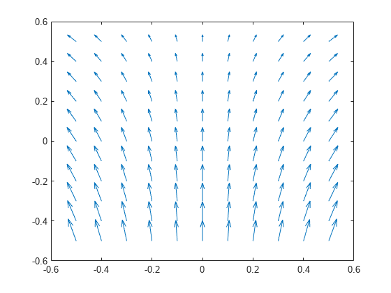
Create a grid specified by x and y coordinates, and evaluate heat flux to the grid.
v = linspace(-0.5,0.5,11);
[X,Y] = meshgrid(v);
[qx,qy] = evaluateHeatFlux(R,X,Y);
Reshape the qTx and qTy vectors, and plot the resulting heat flux.
qx = reshape(qx,size(X));
qy = reshape(qy,size(Y));
figure
quiver(X,Y,qx,qy)
Alternatively, you can specify the grid by using a matrix of query points.
querypoints = [X(:) Y(:)]';
[qx,qy] = evaluateHeatFlux(R,querypoints);

qx = reshape(qx,size(X));
qy = reshape(qy,size(Y));
figure
quiver(X,Y,qx,qy)

For a 3-D steady-state thermal problem, evaluate heat flux at the nodal locations and at the points specified by x, y, and z coordinates.
Create an femodel object for steady-state thermal analysis and include a block geometry in the model.
model = femodel(AnalysisType="thermalSteady", ...
                Geometry="Block.stl");
Plot the geometry.
pdegplot(model.Geometry,FaceLabels="on",FaceAlpha=0.5)
title("Copper block, cm")
axis equal
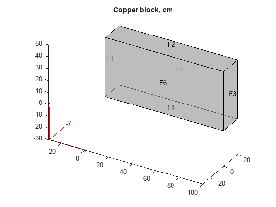
Assuming that this is a copper block, the thermal conductivity of the block is approximately .
model.MaterialProperties = ...
    materialProperties(ThermalConductivity=4);
Apply a constant temperature of 373 K to the left side of the block (face 1) and a constant temperature of 573 K to the right side of the block (face 3).
model.FaceBC(1) = faceBC(Temperature=373);
model.FaceBC(3) = faceBC(Temperature=573);
Apply a heat flux boundary condition to the bottom of the block.
model.FaceLoad(4) = faceLoad(Heat=-20);
Mesh the geometry and solve the problem.
model = generateMesh(model);
R = solve(model)
R =
  SteadyStateThermalResults with properties:

    Temperature: [12822×1 double]
     XGradients: [12822×1 double]
     YGradients: [12822×1 double]
     ZGradients: [12822×1 double]
           Mesh: [1×1 FEMesh]
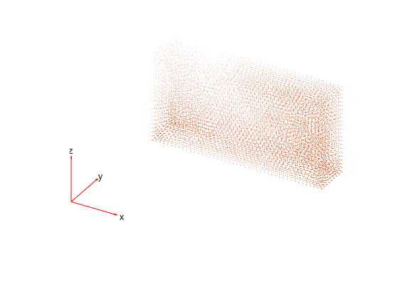
Evaluate heat flux at the nodal locations.
[qx,qy,qz] = evaluateHeatFlux(R);

figure
pdeplot3D(R.Mesh,FlowData=[qx qy qz])
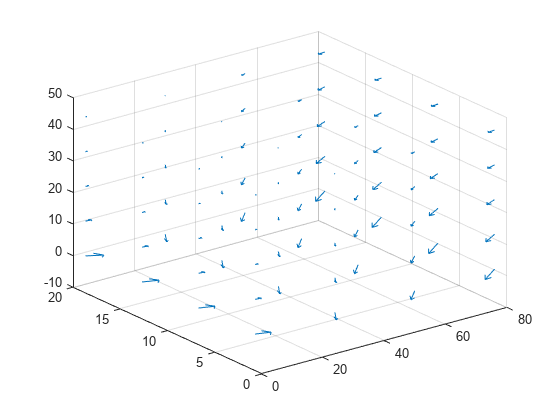
Create a grid specified by x, y, and z coordinates, and evaluate heat flux to the grid.
[X,Y,Z] = meshgrid(1:26:100,1:6:20,1:11:50);

[qx,qy,qz] = evaluateHeatFlux(R,X,Y,Z);
Reshape the qx, qy, and qz vectors, and plot the resulting heat flux.
qx = reshape(qx,size(X));
qy = reshape(qy,size(Y));
qz = reshape(qz,size(Z));
figure
quiver3(X,Y,Z,qx,qy,qz)

Alternatively, you can specify the grid by using a matrix of query points.
querypoints = [X(:) Y(:) Z(:)]';
[qx,qy,qz] = evaluateHeatFlux(R,querypoints);

qx = reshape(qx,size(X));
qy = reshape(qy,size(Y));
qz = reshape(qz,size(Z));
figure
quiver3(X,Y,Z,qx,qy,qz)
Solve a 2-D transient heat transfer problem on a square domain, and compute heat flow across a convective boundary.
Create an femodel object for transient thermal analysis and include a unit square geometry into the model.
model = femodel(AnalysisType="thermalTransient", ...
                Geometry=@squareg);
Plot the geometry.
pdegplot(model.Geometry,EdgeLabels="on")
xlim([-1.1 1.1])
ylim([-1.1 1.1])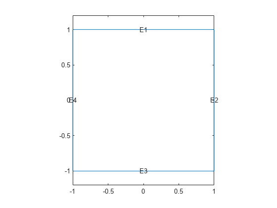
Assign the following thermal properties: thermal conductivity is , mass density is , and specific heat is .
model.MaterialProperties = ...
    materialProperties(ThermalConductivity=100,...
                       MassDensity=7800,...
                       SpecificHeat=500);
Apply the convection boundary condition on the right edge.
model.EdgeLoad(2) = ...
    edgeLoad(ConvectionCoefficient=5000,...
             AmbientTemperature=25);
Set the initial conditions: uniform room temperature across domain and higher temperature on the top edge.
model.FaceIC = faceIC(Temperature=25);
model.EdgeIC(1) = edgeIC(Temperature=100);
Generate a mesh and solve the problem using 0:1000:200000 as a vector of times.
model = generateMesh(model);
tlist = 0:1000:200000;
R = solve(model,tlist);
Create a grid specified by x and y coordinates, and evaluate heat flux to the grid.
v = linspace(-1,1,11);
[X,Y] = meshgrid(v);

[qx,qy] = evaluateHeatFlux(R,X,Y,1:length(tlist));
Reshape qx and qy, and plot the resulting heat flux for the 25th solution step.
tlist(25)
ans =
24000
figure
quiver(X(:),Y(:),qx(:,25),qy(:,25));
xlim([-1,1])
axis equal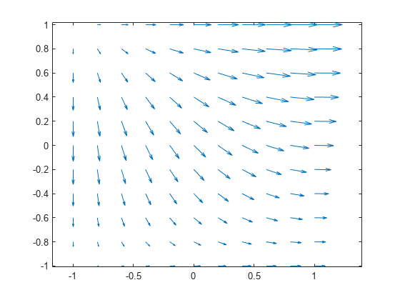
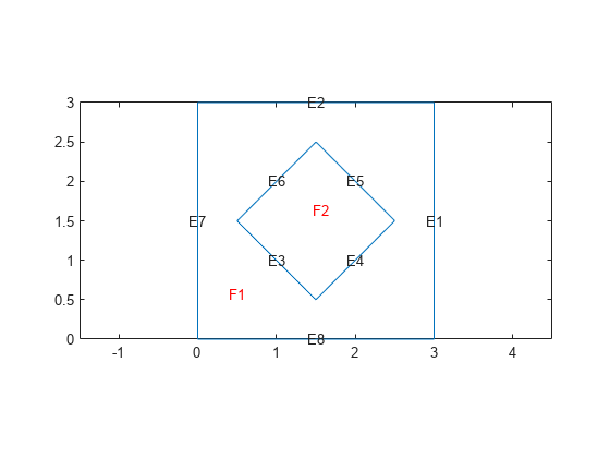
Solve the heat transfer problem for the 2-D geometry consisting of a square and a diamond made of different materials. Compute the heat flux, and plot it as a vector field.
Create and plot the geometry.
SQ1 = [3; 4; 0; 3; 3; 0; 0; 0; 3; 3];
D1 = [2; 4; 0.5; 1.5; 2.5; 1.5; 1.5; 0.5; 1.5; 2.5];
gd = [SQ1 D1];
sf = 'SQ1+D1';
ns = char('SQ1','D1');
ns = ns';
g = decsg(gd,sf,ns);
pdegplot(g,EdgeLabels="on",FaceLabels="on")
xlim([-1.5 4.5])
ylim([-0.5 3.5])
Create an femodel object for transient thermal analysis and include the geometry into the model.
model = femodel(AnalysisType="thermalTransient", ...
                Geometry=g);
For the square region, assign these thermal properties: thermal conductivity is , mass density is , and specific heat is .
model.MaterialProperties(1) = ...
    materialProperties(ThermalConductivity=10,...
                       MassDensity=2,...
                       SpecificHeat=0.1);
For the diamond-shaped region, assign the following thermal properties: thermal conductivity is , mass density is , and specific heat is .
model.MaterialProperties(2) = ...
    materialProperties(ThermalConductivity=2,...
                       MassDensity=1,...
                       SpecificHeat=0.1);
Assume that the diamond-shaped region is a heat source with the density of .
model.FaceLoad(2) = faceLoad(Heat=4);
Apply a constant temperature of to the sides of the square plate.
model.EdgeBC(1:4) = edgeBC(Temperature=0);
Set the initial temperature to .
model.FaceIC = faceIC(Temperature=0);
Generate a mesh.
model = generateMesh(model);
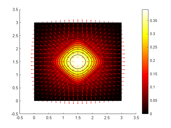
The dynamic for this problem is very fast: the temperature reaches steady state in about 0.1 seconds. To capture the interesting part of the dynamics, set the solution time to logspace(-2,-1,10). This gives 10 logarithmically spaced solution times between 0.01 and 0.1. Solve the problem.
tlist = logspace(-2,-1,10);
R = solve(model,tlist);
temp = R.Temperature;
Compute the heat flux density. Plot the solution with isothermal lines using a contour plot, and plot the heat flux vector field using arrows.
[qTx,qTy] = evaluateHeatFlux(R);

figure
pdeplot(R.Mesh,XYData=temp(:,10), ...
        FlowData=[qTx(:,10) qTy(:,10)], ...
        Contour="on",ColorMap="hot")
axis equal
Input Arguments
Output Arguments
Version History
Introduced in R2017a