readgeotable
Description
T = readgeotable(filename)
T = readgeotable(filename,Name=Value)CoordinateSystemType name-value argument.
Examples
Read a shapefile, containing a network of roads in Concord, MA, into the workspace as a geospatial table.
T = readgeotable("concord_roads.shp");The Shape variable of the table contains information about the road shapes, including the coordinate reference system (CRS). The road shapes in this shapefile use a projected CRS. Prepare to create a map by setting the projected CRS to a variable.
pcrs = T.Shape.ProjectedCRS
pcrs =
  projcrs with properties:

                    Name: "NAD83 / Massachusetts Mainland"
           GeographicCRS: [1×1 geocrs]
        ProjectionMethod: "Lambert Conic Conformal (2SP)"
              LengthUnit: "meter"
    ProjectionParameters: [1×1 map.crs.ProjectionParameters]
Set up a map using the projected CRS. Display the roads on the map.
figure
newmap(pcrs)
geoplot(T)

An optional projection file (.prj) determines the coordinate system type for a shapefile. When your shapefile does not have a projection file, but you know the coordinate system type, you can specify it by using the CoordinateSystemType name-value argument.
Read a shapefile called tsunamis.shp, containing information about tsunami events, into the workspace. The metadata accompanying the file indicates that the shapefile uses geographic coordinates.
T = readgeotable("tsunamis.shp",CoordinateSystemType="geographic");
View the Shape variable of the geospatial table. The tsunami source locations are stored as points.
T.Shape
ans =
  162×1 geopointshape array with properties:

               NumPoints: [162×1 double]
                Latitude: [162×1 double]
               Longitude: [162×1 double]
                Geometry: "point"
    CoordinateSystemType: "geographic"
           GeographicCRS: []
Plot the source locations on a map.
lat = T.Shape.Latitude;
lon = T.Shape.Longitude;
geoiconchart(lat,lon)

GPX files can contain up to five layers: waypoints, tracks, track points, routes, and route points. When you read a layer containing track points or route points, the geospatial table contains an ID variable that associates the points with a track or route.
Import the tracks layer of a GPX file with two tracks. The Shape variable for each track is a geolineshape object.
T = readgeotable("sample_tracks.gpx",Layer="tracks")
T=2×3 table
       Shape                                                  Name                                               Number
    ____________    _________________________________________________________________________________________    ______

    geolineshape    "Track logs from walking the perimeter of the MathWorks campus in Natick on May 21, 2007"      1
    geolineshape    "Track logs from biking from Concord to the MathWorks campus in Natick on June 30, 2011"       2
View the shape of each track. The first track has one segment and the second track has five segments.
T.Shape(1)
ans =
  geolineshape with properties:

                NumParts: 1
                Geometry: "line"
    CoordinateSystemType: "geographic"
           GeographicCRS: [1×1 geocrs]
T.Shape(2)
ans =
  geolineshape with properties:

                NumParts: 5
                Geometry: "line"
    CoordinateSystemType: "geographic"
           GeographicCRS: [1×1 geocrs]
Import the track points layer. The Shape variable for each point is a geopointshape object.
T2 = readgeotable("sample_tracks.gpx",Layer="track_points");
T2.Shape
ans =
  2586×1 geopointshape array with properties:

               NumPoints: [2586×1 double]
                Latitude: [2586×1 double]
               Longitude: [2586×1 double]
                Geometry: "point"
    CoordinateSystemType: "geographic"
           GeographicCRS: [1×1 geocrs]
Create a subtable that contains points in the second track only. For this file, points in the second track have a TrackFID value of 1.
rows = (T2.TrackFID == 1);
T3 = T2(rows,:);
Display the points in the subtable using a blue line.
lat = T3.Shape.Latitude;
lon = T3.Shape.Longitude;
geoplot(lat,lon,Color="b")
Read GeoJSON data from a website and save it in the file storms.geojson. The data contains day 1 convective outlooks from the NOAA/NWS Storm Prediction Center. For more information about convective outlooks, see [1]. For links to the data, see [2].
websave("storms.geojson","https://www.spc.noaa.gov/products/outlook/day1otlk_cat.lyr.geojson");
Read the data into a geospatial table. If the file contains no data for the readgeotable function to read, such as when there are no severe thunderstorm threats, create a geospatial table with an empty polygon shape instead.
try
    GT = readgeotable("storms.geojson");
catch
    GT = table(geopolyshape,"No Data","none",VariableNames=["Shape" "LABEL2" "fill"]);
end
View the Shape variable of the geospatial table. The table stores the geographic areas as polygons.
GT.Shape
ans=2×1 geopolyshape array with properties:
              NumRegions: [2×1 double]
                NumHoles: [2×1 double]
                Geometry: "polygon"
    CoordinateSystemType: "geographic"
           GeographicCRS: [1×1 geocrs]
Day 1 convective outlooks change from day to day, so your results can be different.
Display the convective outlooks over a satellite basemap. To create a legend from the thunderstorm risk categories, plot each row of the table as a separate polygon.
figure
geobasemap satellite
hold on
for k = 1:height(GT)
    row = GT(k,:);
    geoplot(row,"DisplayName",row.LABEL2,"FaceColor",row.fill)
end
legend
alpha(0.6)
Add a title, including the access date.
dt = datetime("today",Format="MMMM d, yyyy");
title("Day 1 Convective Outlooks",string(dt))

[1] "SPC Products." NOAA/National Weather Service Storm Prediction Center. Accessed June 28, 2022. https://www.spc.noaa.gov/misc/about.html.
[2] "SPC Shapefile/KML/KMZ Links." NOAA/National Weather Service Storm Prediction Center. Accessed June 28, 2022. https://www.spc.noaa.gov/gis/.
Since R2023b
OpenStreetMap® files contain several data layers, including point, line, multilinestring, and multipolygon layers. The data that the readgeotable function reads from an OpenStreetMap file depends on the layer that you specify.
Specify the name of an OpenStreetMap file [1] containing data for several city blocks in Shibuya, Tokyo, Japan.
filename = "shibuya.osm";Read the lines layer into a geospatial table. The lines layer represents features such as roads, sidewalks, and railroad tracks. The table represents the lines using line shapes in geographic coordinates.
linesLayer = readgeotable(filename,Layer="lines");Display the lines on a map.
figure
geoplot(linesLayer)
title("Lines Layer")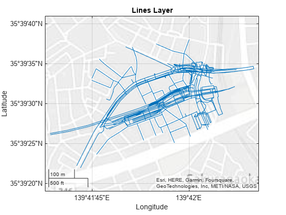
Read the points layer into a geospatial table. The points layer represents features such as traffic signals, bus stops, and subway entrances. The table represents the points using point shapes in geographic coordinates.
pointsLayer = readgeotable(filename,Layer="points");Display the points on the same map.
hold on
geoplot(pointsLayer)
title("Points and Lines Layers")

For information on how to read specific geographic features, such as railways and subway entrances, see the Read Data from OpenStreetMap Files example.
[1] You can download OpenStreetMap files from https://www.openstreetmap.org, which provides access to crowd-sourced map data all over the world. The data is licensed under the Open Data Commons Open Database License (ODbL), https://opendatacommons.org/licenses/odbl/.
Since R2023b
Read buildings data, such as footprints, centroids, and heights, from OpenStreetMap files with the .osm extension.
Specify the name of an OpenStreetMap file [1] containing data for several city blocks in Shibuya, Tokyo, Japan.
filename = "shibuya.osm";Read the buildings layer into a geospatial table by specifying the Layer name-value argument of the readgeotable function as "buildings". The table represents the buildings using polygon shapes in geographic coordinates.
buildingsLayer = readgeotable(filename,Layer="buildings");Display the buildings on a map, and apply color using the maximum heights of the buildings. Add a title, change the colormap, and add a labeled color bar.
figure
geoplot(buildingsLayer,ColorVariable="MaxHeight")

title("Maximum Heights of Buildings")
colormap sky
c = colorbar;
c.Label.String = "Height in Meters";

For information on how to display buildings data based on information stored in the geospatial table, see the Display Buildings from OpenStreetMap Files example.
[1] You can download OpenStreetMap files from https://www.openstreetmap.org, which provides access to crowd-sourced map data all over the world. The data is licensed under the Open Data Commons Open Database License (ODbL), https://opendatacommons.org/licenses/odbl/.