paretosearch

Find points in Pareto set

Syntax

x = paretosearch(fun,nvars)

x = paretosearch(fun,nvars,A,b)

x = paretosearch(fun,nvars,A,b,Aeq,beq)

x = paretosearch(fun,nvars,A,b,Aeq,beq,lb,ub)

x = paretosearch(fun,nvars,A,b,Aeq,beq,lb,ub,nonlcon)

x = paretosearch(fun,nvars,A,b,Aeq,beq,lb,ub,nonlcon,options)

x = paretosearch(problem)

[x,fval] = paretosearch(___)

[x,fval,exitflag,output] = paretosearch(___)

[x,fval,exitflag,output,residuals] = paretosearch(___)

Description

x = paretosearch(fun,nvars) finds nondominated points of the multiobjective function fun. The nvars argument is the dimension of the optimization problem (number of decision variables).

x = paretosearch(fun,nvars,A,b) finds nondominated points subject to the linear inequalities A*x ≤ b. See Linear Inequality Constraints.

x = paretosearch(fun,nvars,A,b,Aeq,beq) finds nondominated points subject to the linear constraints Aeq*x = beq and A*x ≤ b. If no linear inequalities exist, set A = [] and b = [].

x = paretosearch(fun,nvars,A,b,Aeq,beq,lb,ub) defines a set of lower and upper bounds on the design variables in x, so that x is always in the range lb ≤ x ≤ ub. If no linear equalities exist, set Aeq = [] and beq = []. If x(i) has no lower bound, set lb(i) = -Inf. If x(i) has no upper bound, set ub(i) = Inf.

x = paretosearch(fun,nvars,A,b,Aeq,beq,lb,ub,nonlcon) applies the nonlinear inequalities c(x) defined in nonlcon. The paretosearch function finds nondominated points such that c(x) ≤ 0. If no bounds exist, set lb = [], ub = [], or both.

Note

Currently, paretosearch does not support nonlinear equality constraints ceq(x) = 0.

x = paretosearch(fun,nvars,A,b,Aeq,beq,lb,ub,nonlcon,options) finds nondominated points with the optimization options specified in options. Use optimoptions to set these options. If there are no nonlinear inequality or equality constraints, set nonlcon = [].

x = paretosearch(problem) finds the nondominated points for problem, where problem is a structure described in problem.

[x,fval] = paretosearch(___), for any input variables, returns the matrix fval, the value of all the objective functions in fun for all the solutions (rows) in x. The output fval has nf columns, where nf is the number of objectives, and has the same number of rows as x.

[x,fval,exitflag,output] = paretosearch(___) also returns exitflag, an integer identifying the reason the algorithm stopped, and output, a structure that contains information about the solution process.

[x,fval,exitflag,output,residuals] = paretosearch(___) also returns residuals, a structure containing the constraint values at the solution points x.

Examples

Find Pareto Front

Find points on the Pareto front of a two-objective function of a two-dimensional variable.

fun = @(x)[norm(x-[1,2])^2;norm(x+[2,1])^2];
rng default % For reproducibility
x = paretosearch(fun,2);

Pareto set found that satisfies the constraints. 

Optimization completed because the relative change in the volume of the Pareto set 
is less than 'options.ParetoSetChangeTolerance' and constraints are satisfied to within 
'options.ConstraintTolerance'.

Plot the solution as a scatter plot.

plot(x(:,1),x(:,2),'m*')
xlabel('x(1)')
ylabel('x(2)')

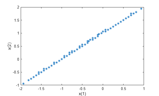
Theoretically, the solution of this problem is a straight line from [-2,-1] to [1,2]. paretosearch returns evenly-spaced points close to this line.

Create Pareto Front with Linear Constraints

Create a Pareto front for a two-objective problem in two dimensions subject to the linear constraint x(1) + x(2) <= 1.

fun = @(x)[norm(x-[1,2])^2;norm(x+[2,1])^2];
A = [1,1];
b = 1;
rng default % For reproducibility
x = paretosearch(fun,2,A,b);

Pareto set found that satisfies the constraints. 

Optimization completed because the relative change in the volume of the Pareto set 
is less than 'options.ParetoSetChangeTolerance' and constraints are satisfied to within 
'options.ConstraintTolerance'.

Plot the solution as a scatter plot.

plot(x(:,1),x(:,2),'m*')
xlabel('x(1)')
ylabel('x(2)')

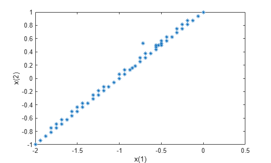
Theoretically, the solution of this problem is a straight line from [-2,-1] to [0,1]. paretosearch returns evenly-spaced points close to this line.

Create Pareto Front with Bounds

Create a Pareto front for a two-objective problem in two dimensions subject to the bounds x(1) >= 0 and x(2) <= 1.

fun = @(x)[norm(x-[1,2])^2;norm(x+[2,1])^2];
lb = [0,-Inf]; % x(1) >= 0
ub = [Inf,1]; % x(2) <= 1
rng default % For reproducibility
x = paretosearch(fun,2,[],[],[],[],lb,ub);

Pareto set found that satisfies the constraints. 

Optimization completed because the relative change in the volume of the Pareto set 
is less than 'options.ParetoSetChangeTolerance' and constraints are satisfied to within 
'options.ConstraintTolerance'.

Plot the solution as a scatter plot.

plot(x(:,1),x(:,2),'m*')
xlabel('x(1)')
ylabel('x(2)')

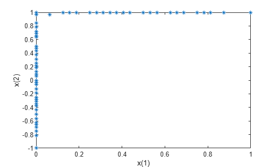
All of the solution points are on the constraint boundaries x(1) = 0 or x(2) = 1.

Create Pareto Front with Nonlinear Constraints

Create a Pareto front for a two-objective problem in two dimensions subject to bounds -1.1 <= x(i) <= 1.1 and the nonlinear constraint norm(x)^2 <= 1.2. The nonlinear constraint function appears at the end of this example, and works if you run this example as a live script. To run this example otherwise, include the nonlinear constraint function as a file on your MATLAB® path.

To better see the effect of the nonlinear constraint, set options to use a large Pareto set size.

rng default % For reproducibility
fun = @(x)[norm(x-[1,2])^2;norm(x+[2,1])^2];
lb = [-1.1,-1.1];
ub = [1.1,1.1];
options = optimoptions('paretosearch','ParetoSetSize',200);
x = paretosearch(fun,2,[],[],[],[],lb,ub,@circlecons,options);

Pareto set found that satisfies the constraints. 

Optimization completed because the relative change in the volume of the Pareto set 
is less than 'options.ParetoSetChangeTolerance' and constraints are satisfied to within 
'options.ConstraintTolerance'.

Plot the solution as a scatter plot. Include a plot of the circular constraint boundary.

figure
plot(x(:,1),x(:,2),'k*')
xlabel('x(1)')
ylabel('x(2)')
hold on
rectangle('Position',[-1.2 -1.2 2.4 2.4],'Curvature',1,'EdgeColor','r')
xlim([-1.2,0.5])
ylim([-0.5,1.2])
axis square
hold off

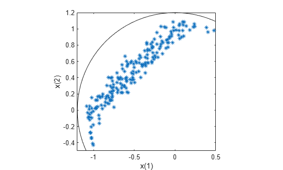
The solution points that have positive x(1) values or negative x(2) values are close to the nonlinear constraint boundary.

function [c,ceq] = circlecons(x)
ceq = [];
c = norm(x)^2 - 1.2;
end

Find Pareto Front Using Options

To monitor the progress of paretosearch, specify the 'psplotparetof' plot function.

fun = @(x)[norm(x-[1,2])^2;norm(x+[2,1])^2];
options = optimoptions('paretosearch','PlotFcn','psplotparetof');
lb = [-4,-4];
ub = -lb;
x = paretosearch(fun,2,[],[],[],[],lb,ub,[],options);

Pareto set found that satisfies the constraints. 

Optimization completed because the relative change in the volume of the Pareto set 
is less than 'options.ParetoSetChangeTolerance' and constraints are satisfied to within 
'options.ConstraintTolerance'.

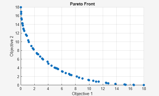
The solution looks like a quarter-circular arc with radius 18, which can be shown to be the analytical solution.

Find Pareto Front in Function Space and Parameter Space

Obtain the Pareto front in both function space and parameter space by calling paretosearch with both the x and fval outputs. Set options to plot the Pareto set in both function space and parameter space.

fun = @(x)[norm(x-[1,2])^2;norm(x+[2,1])^2];
lb = [-4,-4];
ub = -lb;
options = optimoptions('paretosearch','PlotFcn',{'psplotparetof' 'psplotparetox'});
rng default % For reproducibility
[x,fval] = paretosearch(fun,2,[],[],[],[],lb,ub,[],options);

Pareto set found that satisfies the constraints. 

Optimization completed because the relative change in the volume of the Pareto set 
is less than 'options.ParetoSetChangeTolerance' and constraints are satisfied to within 
'options.ConstraintTolerance'.

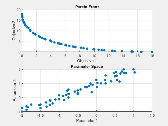
The analytical solution in objective function space is a quarter-circular arc of radius 18. In parameter space, the analytical solution is a straight line from [-2,-1] to [1,2]. The solution points are close to the analytical curves.

Monitor Pareto Set Solution

Set options to monitor the Pareto set solution process. Also, obtain more outputs from paretosearch to enable you to understand the solution process.

options = optimoptions('paretosearch','Display','iter',...
    'PlotFcn',{'psplotparetof' 'psplotparetox'});
fun = @(x)[norm(x-[1,2])^2;norm(x+[2,1])^2];
lb = [-4,-4];
ub = -lb;
rng default % For reproducibility
[x,fval,exitflag,output] = paretosearch(fun,2,[],[],[],[],lb,ub,[],options);

Iter   F-count   NumSolutions  Spread       Volume 
   0        60        11          -         3.7872e+02
   1       386        12       7.6126e-01   3.4654e+02
   2       702        27       9.5232e-01   2.9452e+02
   3      1029        27       6.6332e-02   2.9904e+02
   4      1357        36       1.3874e-01   3.0070e+02
   5      1690        37       1.5379e-01   3.0200e+02
   6      2014        50       1.7828e-01   3.0252e+02
   7      2214        59       1.8536e-01   3.0320e+02
   8      2344        60       1.9435e-01   3.0361e+02
   9      2464        60       2.1055e-01   3.0388e+02

Pareto set found that satisfies the constraints. 

Optimization completed because the relative change in the volume of the Pareto set 
is less than 'options.ParetoSetChangeTolerance' and constraints are satisfied to within 
'options.ConstraintTolerance'.

Examine the additional outputs.

fprintf('Exit flag %d.\n',exitflag)

Exit flag 1.

disp(output)

         iterations: 10
          funccount: 2464
             volume: 303.6076
    averagedistance: 0.0250
             spread: 0.2105
      maxconstraint: 0
            message: 'Pareto set found that satisfies the constraints. ...'
           rngstate: [1x1 struct]

Obtain Pareto Front Residuals

Obtain and examine the Pareto front constraint residuals. Create a problem with the linear inequality constraint sum(x) <= -1/2 and the nonlinear inequality constraint norm(x)^2 <= 1.2. For improved accuracy, use 200 points on the Pareto front, and a ParetoSetChangeTolerance of 1e-7, and give the natural bounds -1.2 <= x(i) <= 1.2.

The nonlinear constraint function appears at the end of this example, and works if you run this example as a live script. To run this example otherwise, include the nonlinear constraint function as a file on your MATLAB® path.

fun = @(x)[norm(x-[1,2])^2;norm(x+[2,1])^2];
A = [1,1];
b = -1/2;
lb = [-1.2,-1.2];
ub = -lb;
nonlcon = @circlecons;
rng default % For reproducibility
options = optimoptions('paretosearch','ParetoSetChangeTolerance',1e-7,...
    'PlotFcn',{'psplotparetof' 'psplotparetox'},'ParetoSetSize',200);

Call paretosearch using all outputs.

[x,fval,exitflag,output,residuals] = paretosearch(fun,2,A,b,[],[],lb,ub,nonlcon,options);

Pareto set found that satisfies the constraints. 

Optimization completed because the relative change in the volume of the Pareto set 
is less than 'options.ParetoSetChangeTolerance' and constraints are satisfied to within 
'options.ConstraintTolerance'.

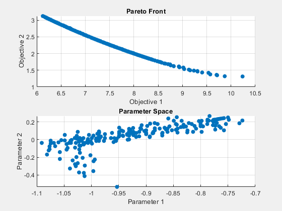
The inequality constraints reduce the size of the Pareto set compared to an unconstrained set. Examine the returned residuals.

fprintf('The maximum linear inequality constraint residual is %f.\n',max(residuals.ineqlin))

The maximum linear inequality constraint residual is 0.000000.

fprintf('The maximum nonlinear inequality constraint residual is %f.\n',max(residuals.ineqnonlin))

The maximum nonlinear inequality constraint residual is -0.000537.

The maximum returned residuals are negative, meaning that all the returned points are feasible. The maximum returned residuals are close to zero, meaning that each constraint is active for some points.

function [c,ceq] = circlecons(x)
ceq = [];
c = norm(x)^2 - 1.2;
end

Input Arguments

fun — Objective functions to optimize

function handle | function name

Objective functions to optimize, specified as a function handle or function name.

fun is a function that accepts a real row vector of doubles x of length nvars and returns a real vector F(x) of objective function values. For details on writing fun, see Compute Objective Functions.

If you set the UseVectorized option to true, then fun accepts a matrix of size n-by-nvars, where the matrix represents n individuals. fun returns a matrix of size n-by-m, where m is the number of objective functions. See Vectorize the Fitness Function.

Example: @(x)[sin(x),cos(x)]

Data Types: char | function_handle | string

nvars — Number of variables

positive integer

Number of variables, specified as a positive integer. The solver passes row vectors of length nvars to fun.

Example: 4

Data Types: double

A — Linear inequality constraints

real matrix

Linear inequality constraints, specified as a real matrix. A is an M-by-nvars matrix, where M is the number of inequalities.

A encodes the M linear inequalities

A*x <= b,

where x is the column vector of nvars variables x(:), and b is a column vector with M elements.

For example, to specify

x₁ + 2x₂ ≤ 10
3x₁ + 4x₂ ≤ 20
5x₁ + 6x₂ ≤ 30,

give these constraints:

A = [1,2;3,4;5,6];
b = [10;20;30];

Example: To specify that the control variables sum to 1 or less, give the constraints A = ones(1,N) and b = 1.

Data Types: double

b — Linear inequality constraints

real vector

Linear inequality constraints, specified as a real vector. b is an M-element vector related to the A matrix. If you pass b as a row vector, solvers internally convert b to the column vector b(:).

b encodes the M linear inequalities

A*x <= b,

where x is the column vector of N variables x(:), and A is a matrix of size M-by-N.

For example, to specify

x₁ + 2x₂ ≤ 10
3x₁ + 4x₂ ≤ 20
5x₁ + 6x₂ ≤ 30,

give these constraints:

A = [1,2;3,4;5,6];
b = [10;20;30];

Example: To specify that the control variables sum to 1 or less, give the constraints A = ones(1,N) and b = 1.

Data Types: double

Aeq — Linear equality constraints

real matrix

Linear equality constraints, specified as a real matrix. Aeq is an Me-by-nvars matrix, where Me is the number of equalities.

Aeq encodes the Me linear equalities

Aeq*x = beq,

where x is the column vector of N variables x(:), and beq is a column vector with Me elements.

For example, to specify

x₁ + 2x₂ + 3x₃ = 10
2x₁ + 4x₂ + x₃ = 20,

give these constraints:

Aeq = [1,2,3;2,4,1];
beq = [10;20];

Example: To specify that the control variables sum to 1, give the constraints Aeq = ones(1,N) and beq = 1.

Data Types: double

beq — Linear equality constraints

real vector

Linear equality constraints, specified as a real vector. beq is an Me-element vector related to the Aeq matrix. If you pass beq as a row vector, solvers internally convert beq to the column vector beq(:).

beq encodes the Me linear equalities

Aeq*x = beq,

where x is the column vector of N variables x(:), and Aeq is a matrix of size Meq-by-N.

For example, to specify

x₁ + 2x₂ + 3x₃ = 10
2x₁ + 4x₂ + x₃ = 20,

give these constraints:

Aeq = [1,2,3;2,4,1];
beq = [10;20];

Example: To specify that the control variables sum to 1, give the constraints Aeq = ones(1,N) and beq = 1.

Data Types: double

lb — Lower bounds

[] (default) | real vector or array

Lower bounds, specified as a real vector or array of doubles. lb represents the lower bounds element-wise in lb ≤ x ≤ ub.

Internally, paretosearch converts an array lb to the vector lb(:).

Example: lb = [0;-Inf;4] means x(1) ≥ 0, x(3) ≥ 4.

Data Types: double

ub — Upper bounds

[] (default) | real vector or array

Upper bounds, specified as a real vector or array of doubles. ub represents the upper bounds element-wise in lb ≤ x ≤ ub.

Internally, paretosearch converts an array ub to the vector ub(:).

Example: ub = [Inf;4;10] means x(2) ≤ 4, x(3) ≤ 10.

Data Types: double

nonlcon — Nonlinear constraints

function handle | function name

Nonlinear constraints, specified as a function handle or function name. nonlcon is a function that accepts a row vector x and returns two row vectors, c(x) and ceq(x).

• c(x) is the row vector of nonlinear inequality constraints at x. The paretosearch function attempts to satisfy c(x) <= 0 for all entries of c.

• ceq(x) must return [], because currently paretosearch does not support nonlinear equality constraints.

If you set the UseVectorized option to true, then nonlcon accepts a matrix of size n-by-nvars, where the matrix represents n individuals. nonlcon returns a matrix of size n-by-mc in the first argument, where mc is the number of nonlinear inequality constraints. See Vectorize the Fitness Function.

For example, x = paretosearch(@myfun,nvars,A,b,Aeq,beq,lb,ub,@mycon), where mycon is a MATLAB^® function such as the following:

function [c,ceq] = mycon(x)
c = ...     % Compute nonlinear inequalities at x.
ceq = []    % No nonlinear equalities at x.

For more information, see Nonlinear Constraints.

Data Types: char | function_handle | string

options — Optimization options

output of optimoptions | structure

Optimization options, specified as the output of optimoptions or as a structure.

{} denotes the default value. See option details in Pattern Search Options.

Options for paretosearch

Option	Description	Values
ConstraintTolerance	Tolerance on constraints. For an options structure, use TolCon.	Nonnegative scalar | {1e-6}
Display	Level of display.	'off' | 'iter' | 'diagnose' | {'final'}
InitialPoints	Initial points for paretosearch. Use one of these data types: Matrix with nvars columns, where each row represents one initial point. Structure containing the following fields (all fields are optional except X0): X0 — Matrix with nvars columns, where each row represents one initial point. Fvals — Matrix with numObjectives columns, where each row represents the objective function values at the corresponding point in X0. Cineq — Matrix with numIneq columns, where each row represents the nonlinear inequality constraint values at the corresponding point in X0. paretosearch computes any missing values in the Fvals and Cineq fields.	Matrix with nvars columns | structure | {[]}
MaxFunctionEvaluations	Maximum number of objective function evaluations. For an options structure, use MaxFunEvals.	Nonnegative integer | {'2000*numberOfVariables'} for patternsearch, {'3000*(numberOfVariables+numberOfObjectives)'} for paretosearch, where numberOfVariables is the number of problem variables, and numberOfObjectives is the number of objective functions
MaxIterations	Maximum number of iterations. For an options structure, use MaxIter.	Nonnegative integer | {'100*numberOfVariables'} for patternsearch, {'100*(numberOfVariables+numberOfObjectives)'} for paretosearch, where numberOfVariables is the number of problem variables, and numberOfObjectives is the number of objective functions
MaxTime	Total time (in seconds) allowed for optimization. For an options structure, use TimeLimit.	Nonnegative scalar | {Inf}
MeshTolerance	Tolerance on the mesh size. For an options structure, use TolMesh.	Nonnegative scalar | {1e-6}
MinPollFraction	Minimum fraction of the pattern to poll.	Scalar from 0 through 1 | {0}
OutputFcn	Function that an optimization function calls at each iteration. Specify as a function handle or a cell array of function handles. For an options structure, use OutputFcns.	Function handle or cell array of function handles | {[]}
ParetoSetChangeTolerance	The solver stops when the relative change in a stopping measure over a window of iterations is less than or equal to ParetoSetChangeTolerance. For three or fewer objectives, paretosearch uses the volume and spread measures. For four or more objectives, paretosearch uses the spread and distance measures. See Definitions for paretosearch Algorithm. The solver stops when the relative change in any applicable measure is less than ParetoSetChangeTolerance, or the maximum of the squared Fourier transforms of the time series of these measures is relatively small. See paretosearch Algorithm. Note Setting ParetoSetChangeTolerance < sqrt(eps) ~ 1.5e-8 is not recommended.	Nonnegative scalar | {1e-4}
ParetoSetSize	Number of points in the Pareto set.	Positive integer | {'max(numberOfObjectives, 60)'}, where numberOfObjectives is the number of objective functions
PlotFcn	Plots of output from the pattern search. Specify as the name of a built-in plot function, a function handle, or a cell array of names of built-in plot functions or function handles. For an options structure, use PlotFcns.	{[]} | 'psplotfuncount' | 'psplotmaxconstr' | custom plot function With multiple objectives: 'psplotdistance' | 'psplotparetof' | 'psplotparetox' | 'psplotspread' | 'psplotvolume' With a single objective: 'psplotbestf' | 'psplotmeshsize' | 'psplotbestx'
PollMethod	Polling strategy used in the pattern search. Note You cannot use MADS polling when the problem has linear equality constraints.	{'GPSPositiveBasis2np2'} | 'GPSPositiveBasis2N' | 'GPSPositiveBasisNp1' | 'GSSPositiveBasis2N' | 'GSSPositiveBasisNp1' | 'MADSPositiveBasis2N' | 'MADSPositiveBasisNp1' | 'GSSPositiveBasis2np2'
UseParallel	Compute objective and nonlinear constraint functions in parallel. See Vectorized and Parallel Options and How to Use Parallel Processing in Global Optimization Toolbox. Note You must set UseCompletePoll to true for patternsearch to use vectorized or parallel polling. Similarly, set UseCompleteSearch to true for vectorized or parallel searching. Beginning in R2019a, when you set the UseParallel option to true, patternsearch internally overrides the UseCompletePoll setting to true so that the function polls in parallel.	true | {false}
UseVectorized	Specifies whether functions are vectorized. See Vectorized and Parallel Options and Vectorize the Objective and Constraint Functions. Note You must set UseCompletePoll to true for patternsearch to use vectorized or parallel polling. Similarly, set UseCompleteSearch to true for vectorized or parallel searching. For an options structure, use Vectorized = 'on' or 'off'.	true | {false}

Example: options = optimoptions('paretosearch','Display','none','UseParallel',true)

problem — Problem structure

structure

Problem structure, specified as a structure with the following fields:

• objective — Objective function

• nvars — Number of variables

• Aineq — Matrix for linear inequality constraints

• bineq — Vector for linear inequality constraints

• Aeq — Matrix for linear equality constraints

• beq — Vector for linear equality constraints

• lb — Lower bound for x

• ub — Upper bound for x

• nonlcon — Nonlinear constraint function

• solver — 'paretosearch'

• options — Options created with optimoptions

• rngstate — Optional field to reset the state of the random number generator

Note

All fields in problem are required, except for rngstate, which is optional.

Data Types: struct

Output Arguments

x — Pareto points

m-by-nvars array

Pareto points, returned as an m-by-nvars array, where m is the number of points on the Pareto front. Each row of x represents one point on the Pareto front.

fval — Function values on Pareto front

m-by-nf array

Function values on the Pareto front, returned as an m-by-nf array. m is the number of points on the Pareto front, and nf is the number of objective functions. Each row of fval represents the function values at one Pareto point in x.

exitflag — Reason paretosearch stopped

integer

Reason paretosearch stopped, returned as one of the integer values in this table.

Exit Flag	Stopping Condition
1	One of the following conditions is met. Mesh size of all incumbents is less than options.MeshTolerance and constraints (if any) are satisfied to within options.ConstraintTolerance. Relative change in the spread of the Pareto set is less than options.ParetoSetChangeTolerance and constraints (if any) are satisfied to within options.ConstraintTolerance. Relative change in the volume of the Pareto set is less than options.ParetoSetChangeTolerance and constraints (if any) are satisfied to within options.ConstraintTolerance.
0	Number of iterations exceeds options.MaxIterations, or the number of function evaluations exceeds options.MaxFunctionEvaluations.
-1	Optimization is stopped by an output function or plot function.
-2	Solver cannot find a point satisfying all the constraints.
-5	Optimization time exceeds options.MaxTime.

output — Information about the optimization process

structure

Information about the optimization process, returned as a structure with these fields:

• iterations — Total number of iterations.

• funccount — Total number of function evaluations.

• volume — Hyper-volume of the set formed from the Pareto points in function space. See Definitions for paretosearch Algorithm.

• averagedistance — Average distance measure of the Pareto points in function space. See Definitions for paretosearch Algorithm.

• spread — Average spread measure of the Pareto points. See Definitions for paretosearch Algorithm.

• maxconstraint — Maximum constraint violation, if any.

• message — Reason why the algorithm terminated.

• rngstate — State of the MATLAB random number generator just before the algorithm starts. You can use the values in rngstate to reproduce the output when you use a random poll method such as 'MADSPositiveBasis2N' or when you use the default quasirandom method of creating the initial population. See Reproduce Results, which discusses the identical technique for ga.

residuals — Constraint residuals at x

structure

Constraint residuals at x, returned as a structure with these fields (a glossary of the field size terms and entries follows the table).

Field Name	Field Size	Entries
lower	m-by-nvars	lb – x
upper	m-by-nvars	x – ub
ineqlin	m-by-ncon	A*x - b
eqlin	m-by-ncon	|Aeq*x - b|
ineqnonlin	m-by-ncon	c(x)

• m — Number of returned points x on the Pareto front

• nvars — Number of control variables

• ncon — Number of constraints of the relevant type (such as number of rows of A or number of returned nonlinear equalities)

• c(x) — Numeric values of the nonlinear constraint functions

More About

Nondominated

Nondominated points, also called noninferior points, are points for which no other point has lower values of all objective functions. In other words, for nondominated points, none of the objective function values can be improved (lowered) without raising other objective function values. See What Is Multiobjective Optimization?.

Algorithms

paretosearch uses a pattern search to search for points on the Pareto front. For details, see paretosearch Algorithm.

Alternative Functionality

App

The Optimize Live Editor task provides a visual interface for paretosearch.

Extended Capabilities

Automatic Parallel Support

Accelerate code by automatically running computation in parallel using Parallel Computing Toolbox™.

To run in parallel, set the 'UseParallel' option to true.

options = optimoptions('solvername','UseParallel',true)

For more information, see How to Use Parallel Processing in Global Optimization Toolbox.

Version History

Introduced in R2018b