Specify Conditional Mean and Variance Models
This example shows how to specify a composite conditional mean and variance model using arima.
Load the Data
Load the NASDAQ data included with the toolbox. Convert the daily close composite index series to a return series.
load Data_EquityIdx
ReturnsTbl = price2ret(DataTable);
T = height(ReturnsTbl);

figure
plot(ReturnsTbl.NASDAQ)
axis tight
title("NASDAQ Daily Returns")
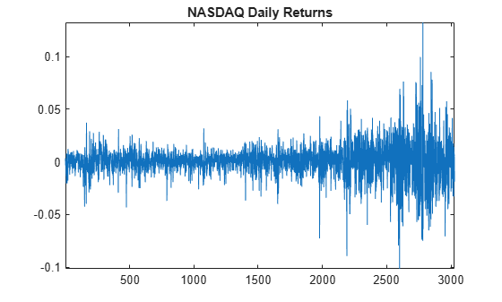
The returns appear to fluctuate around a constant level, but exhibit volatility clustering. Large changes in the returns tend to cluster together, and small changes tend to cluster together. That is, the series exhibits conditional heteroscedasticity.
The returns are of relatively high frequency. Therefore, the daily changes can be small. For numerical stability, it is good practice to scale such data.
Scale the series by 100 and center the percentage returns.
ReturnsTbl.Residuals_NASDAQ = 100*(ReturnsTbl.NASDAQ - mean(ReturnsTbl.NASDAQ));
Check for Autocorrelation
Plot the sample autocorrelation function (ACF) and partial autocorrelation function (PACF) for the residual series. Adjust the -axes of the plots to remedy the plot saturation of the lag 0 correlations.
figure
tiledlayout(2,1)
nexttile
autocorr(ReturnsTbl,DataVariable="Residuals_NASDAQ")
h = gca;
h.YLim(end) = 0.15;
nexttile
parcorr(ReturnsTbl,DataVariable="Residuals_NASDAQ")
h = gca;
h.YLim(end) = 0.15;
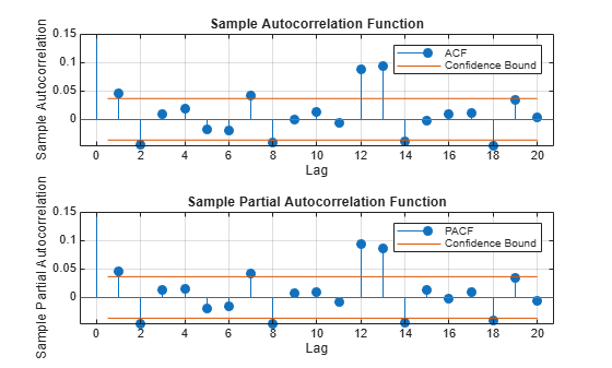
The autocorrelation functions suggests there is significant autocorrelation at lag one and several higher lags.
Test the Significance of Autocorrelations
Conduct a Ljung-Box Q-test at lag 5.
StatTbl = lbqtest(ReturnsTbl,DataVariable="Residuals_NASDAQ",Lags=5)StatTbl=1×7 table
h pValue stat cValue Lags Alpha DoF
_____ ________ ______ ______ ____ _____ ___
Test 1 true 0.011956 14.652 11.07 5 0.05 5
The null hypothesis that all autocorrelations are 0 up to lag 5 is rejected (h = 1).
Check for Conditional Heteroscedasticity.
Plot the sample ACF and PACF of the squared return series.
figure
tiledlayout(2,1)
nexttile
autocorr(ReturnsTbl.Residuals_NASDAQ.^2)
nexttile
parcorr(ReturnsTbl.Residuals_NASDAQ.^2)
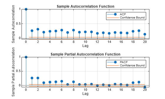
The autocorrelation functions show significant serial dependence, which suggests that the series is conditionally heteroscedastic.
Test for Significant ARCH Effects
Conduct an Engle's ARCH test. Test the null hypothesis of no conditional heteroscedasticity against the alternative hypothesis of an ARCH model with two lags (which is locally equivalent to a GARCH(1,1) model).
StatTbl = archtest(ReturnsTbl,DataVariable="Residuals_NASDAQ",Lags=2)StatTbl=1×6 table
h pValue stat cValue Lags Alpha
_____ ______ ______ ______ ____ _____
Test 1 true 0 399.97 5.9915 2 0.05
The null hypothesis is rejected in favor of the alternative hypothesis (h = 1).
Specify a Conditional Mean and Variance Model.
Specify an AR(1) model for the conditional mean of the centered NASDAQ percentage returns, and a GARCH(1,1) model for the conditional variance. This is a model of the form
where ,
and is an independent and identically distributed standardized Gaussian process.
CondVarMdl = garch(1,1);
Mdl = arima(ARLags=1,Variance=CondVarMdl)
Mdl =
  arima with properties:

     Description: "ARIMA(1,0,0) Model (Gaussian Distribution)"
      SeriesName: "Y"
    Distribution: Name = "Gaussian"
               P: 1
               D: 0
               Q: 0
        Constant: NaN
              AR: {NaN} at lag [1]
             SAR: {}
              MA: {}
             SMA: {}
     Seasonality: 0
            Beta: [1×0]
        Variance: [GARCH(1,1) Model]
The model output shows that a garch model is stored in the Variance property of the arima model, Mdl.