tune
Syntax
Description
[
returns proposal distribution parameter mean vector params,Proposal] = tune(PriorMdl,Y,params0)params and scale
matrix Proposal to improve the Metropolis-Hastings sampler.
PriorMdl is the Bayesian state-space model that specifies the
state-space model structure (likelihood) and prior distribution, Y is
the data for the likelihood, and params0 is the vector of initial
values for the unknown state-space model parameters θ in
PriorMdl.
[
specifies additional options using one or more name-value arguments. For example,
params,Proposal] = tune(PriorMdl,Y,params0,Name=Value)tune(Mdl,Y,params0,Hessian="opg",Display=false) uses the outer-product
of gradients method to compute the Hessian matrix and suppresses the display of the
optimized values.
Examples
Simulate observed responses from a known state-space model, then treat the model as Bayesian and draw parameters from the posterior distribution. Tune the proposal distribution of the Metropolis-Hastings sampler by using tune.
Suppose the following state-space model is a data-generating process (DGP).
Create a standard state-space model object ssm that represents the DGP.
trueTheta = [0.5; -0.75; 1; 0.5];
A = [trueTheta(1) 0; 0 trueTheta(2)];
B = [trueTheta(3) 0; 0 trueTheta(4)];
C = [1 1];
DGP = ssm(A,B,C);
Simulate a response path from the DGP.
rng(1); % For reproducibility
y = simulate(DGP,200);
Suppose the structure of the DGP is known, but the state parameters trueTheta are unknown, explicitly
Consider a Bayesian state-space model representing the model with unknown parameters. Arbitrarily assume that the prior distribution of , , , and are independent Gaussian random variables with mean 0.5 and variance 1.
The Local Functions section contains two functions required to specify the Bayesian state-space model. You can use the functions only within this script.
The paramMap function accepts a vector of the unknown state-space model parameters and returns all the following quantities:
A= .B= .C= .D= 0.Mean0andCov0are empty arrays[], which specify the defaults.StateType= , indicating that each state is stationary.
The paramDistribution function accepts the same vector of unknown parameters as does paramMap, but it returns the log prior density of the parameters at their current values. Specify that parameter values outside the parameter space have log prior density of -Inf.
Create the Bayesian state-space model by passing function handles directly to paramMap and paramDistribution to bssm.
Mdl = bssm(@paramMap,@priorDistribution)
Mdl =
Mapping that defines a state-space model:
    @paramMap

Log density of parameter prior distribution:
    @priorDistribution
The simulate function requires a proposal distribution scale matrix. You can obtain a data-driven proposal scale matrix by using the tune function. Alternatively, you can supply your own scale matrix.
Obtain a data-driven scale matrix by using the tune function. Supply a random set of initial parameter values.
numParams = 4;
theta0 = rand(numParams,1);
[theta0,Proposal] = tune(Mdl,y,theta0);
Local minimum found.

Optimization completed because the size of the gradient is less than
the value of the optimality tolerance.

<stopping criteria details>
         Optimization and Tuning
      | Params0  Optimized  ProposalStd
----------------------------------------
 c(1) |  0.6968    0.4459      0.0798
 c(2) |  0.7662   -0.8781      0.0483
 c(3) |  0.3425    0.9633      0.0694
 c(4) |  0.8459    0.3978      0.0726
theta0 is a 4-by-1 estimate of the posterior mode and Proposal is the Hessian matrix. Both outputs are the optimized moments of the proposal distribution, the latter of which is up to a proportionality constant. tune displays convergence information and an estimation table, which you can suppress by using the Display options of the optimizer and tune.
Draw 1000 random parameter vectors from the posterior distribution. Specify the simulated response path as observed responses and the optimized values returned by tune for the initial parameter values and the proposal distribution.
[Theta,accept] = simulate(Mdl,y,theta0,Proposal);
accept
accept =
0.4010
Theta is a 4-by-1000 matrix of randomly drawn parameters from the posterior distribution. Rows correspond to the elements of the input argument theta of the functions paramMap and priorDistribution.
accept is the proposal acceptance probability. In this case, simulate accepts 40% of the proposal draws.
Local Functions
This example uses the following functions. paramMap is the parameter-to-matrix mapping function and priorDistribution is the log prior distribution of the parameters.
function [A,B,C,D,Mean0,Cov0,StateType] = paramMap(theta)
    A = [theta(1) 0; 0 theta(2)];
    B = [theta(3) 0; 0 theta(4)];
    C = [1 1];
    D = 0;
    Mean0 = [];         % MATLAB uses default initial state mean
    Cov0 = [];          % MATLAB uses initial state covariances
    StateType = [0; 0]; % Two stationary states
end

function logprior = priorDistribution(theta)
    paramconstraints = [(abs(theta(1)) >= 1) (abs(theta(2)) >= 1) ...
        (theta(3) < 0) (theta(4) < 0)];
    if(sum(paramconstraints))
        logprior = -Inf;
    else
        mu0 = 0.5*ones(numel(theta),1);
        sigma0 = 1;
        p = normpdf(theta,mu0,sigma0);
        logprior = sum(log(p));
    end
end
Consider the following time-varying, state-space model for a DGP:
From periods 1 through 250, the state equation includes stationary AR(2) and MA(1) models, respectively, and the observation model is the weighted sum of the two states.
From periods 251 through 500, the state model includes only the first AR(2) model.
and is the identity matrix.
Symbolically, the DGP is
where:
The AR(2) parameters and .
The MA(1) parameter .
The observation equation parameters and .
Write a function that specifies how the parameters theta and sample size T map to the state-space model matrices, the initial state moments, and the state types. Save this code as a file named timeVariantParamMapBayes.m on your MATLAB® path. Alternatively, open the example to access the function.
type timeVariantParamMapBayes.m% Copyright 2022 The MathWorks, Inc.
function [A,B,C,D,Mean0,Cov0,StateType] = timeVariantParamMapBayes(theta,T)
% Time-variant, Bayesian state-space model parameter mapping function
% example. This function maps the vector params to the state-space matrices
% (A, B, C, and D), the initial state value and the initial state variance
% (Mean0 and Cov0), and the type of state (StateType). From periods 1
% through T/2, the state model is a stationary AR(2) and an MA(1) model,
% and the observation model is the weighted sum of the two states. From
% periods T/2 + 1 through T, the state model is the AR(2) model only. The
% log prior distribution enforces parameter constraints (see
% flatPriorBSSM.m).
T1 = floor(T/2);
T2 = T - T1 - 1;
A1 = {[theta(1) theta(2) 0 0; 1 0 0 0; 0 0 0 theta(4); 0 0 0 0]};
B1 = {[theta(3) 0; 0 0; 0 1; 0 1]};
C1 = {theta(5)*[1 0 1 0]};
D1 = {theta(6)};
Mean0 = [0.5 0.5 0 0];
Cov0 = eye(4);
StateType = [0 0 0 0];
A2 = {[theta(1) theta(2) 0 0; 1 0 0 0]};
B2 = {[theta(3); 0]};
A3 = {[theta(1) theta(2); 1 0]};
B3 = {[theta(3); 0]};
C3 = {theta(7)*[1 0]};
D3 = {theta(8)};
A = [repmat(A1,T1,1); A2; repmat(A3,T2,1)];
B = [repmat(B1,T1,1); B2; repmat(B3,T2,1)];
C = [repmat(C1,T1,1); repmat(C3,T2+1,1)];
D = [repmat(D1,T1,1); repmat(D3,T2+1,1)];
end
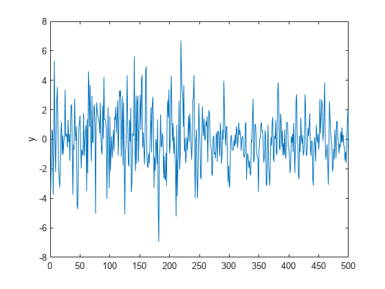
Simulate a response path of length 500 from the model.
params = [0.5; -0.2; 0.4; 0.3; 2; 0.1; 3; 0.2];
numObs = 500;
numParams = numel(params);
[A,B,C,D,mean0,Cov0,stateType] = timeVariantParamMapBayes(params,numObs);
DGP = ssm(A,B,C,D,Mean0=mean0,Cov0=Cov0,StateType=stateType);

rng(1)  % For reproducibility
y = simulate(DGP,numObs);
plot(y)
ylabel("y")
Write a function that specifies a flat prior distribution on the state-space model parameters theta. The function returns the scalar log prior for an input set of parameters. Save this code as a file named flatPriorBSSM.m on your MATLAB® path. Alternatively, open the example to access the function.
type flatPriorBSSM.m% Copyright 2022 The MathWorks, Inc.
function logprior = flatPriorBSSM(theta)
% flatPriorBSSM computes the log of the flat prior density for the eight
% variables in theta (see timeVariantParamMapBayes.m). Log probabilities
% for parameters outside the parameter space are -Inf.
% theta(1) and theta(2) are lag 1 and lag 2 terms in a stationary AR(2)
% model. The eigenvalues of the AR(1) representation need to be within
% the unit circle.
evalsAR2 = eig([theta(1) theta(2); 1 0]);
evalsOutUC = sum(abs(evalsAR2) >= 1) > 0;
% Standard deviations of disturbances and errors (theta(3), theta(6),
% and theta(8)) need to be positive.
nonnegsig1 = theta(3) <= 0;
nonnegsig2 = theta(6) <= 0;
nonnegsig3 = theta(8) <= 0;
paramconstraints = [evalsOutUC nonnegsig1 ...
nonnegsig2 nonnegsig3];
if sum(paramconstraints) > 0
logprior = -Inf;
else
logprior = 0; % Prior density is proportional to 1 for all values
% in the parameter space.
end
end
Create a time-varying, Bayesian state-space model that uses the structure of the DGP.
Mdl = bssm(@(params)timeVariantParamMapBayes(params,numObs),@flatPriorBSSM);
Obtain optimized values for the proposal distribution moments by using tune. Initialize the parameter values to a random set of positive values in [0,0.1]. Suppress all tuning displays. Use the Hessian matrix returned by the optimizer of the posterior mode.
params0 = 0.1*rand(numParams,1);
options = optimoptions("fminunc",Display="off");
[params0,Proposal] = tune(Mdl,y,params0,Options=options,Display=false, ...
    Hessian="optimizer");
Draw a sample from the posterior distribution. Supply the optimized parameter estimates. Set the proposal distribution to multivariate with a scale matrix proportional. Set the proportionality constant to 0.005.
[PostParams,accept] = simulate(Mdl,y,params0,Proposal, ...
    Dof=25,Proportion=0.1);
accept
accept = 0.7880
PostParams is an 8-by-1000 matrix of 1000 random draws from the posterior distribution. The Metropolis-Hastings sampler accepted 80% of the proposed draws.
The log joint prior distribution function specifies parameter constraints by attributing a probability of -Inf for arguments outside the support of the distribution. Because posterior sampling does not occur during proposal distribution tuning, it is good practice to additionally specify constraints when you call tune.
Consider a regression of the US unemployment rate onto and real gross national product (rGNP) rate, and suppose the resulting innovations are an ARMA(1,1) process. The state-space form of the relationship is
where:
is the ARMA process.
is a dummy state for the MA(1) effect.
is the observed unemployment rate deflated by a constant and the rGNP rate ().
is an iid Gaussian series with mean 0 and standard deviation 1.
Load the Nelson-Plosser data set, which contains a table DataTable that has the unemployment rate and rGNP series, among other series.
load Data_NelsonPlosserCreate a variable in DataTable that represents the returns of the raw rGNP series. Because price-to-returns conversion reduces the sample size by one, prepad the series with NaN.
DataTable.RGNPRate = [NaN; price2ret(DataTable.GNPR)];
T = height(DataTable);
Create variables for the regression. Represent the unemployment rate as the observation series and the constant and rGNP rate series as the deflation data .
Z = [ones(T,1) DataTable.RGNPRate];
y = DataTable.UR;
Write a function that specifies how the parameters theta, response series y, and deflation data Z map to the state-space model matrices, the initial state moments, and the state types. Save this code as a file named armaDeflateYBayes.m on your MATLAB® path. Alternatively, open the example to access the function.
type armaDeflateYBayes.m% Copyright 2022 The MathWorks, Inc.
function [A,B,C,D,Mean0,Cov0,StateType,DeflatedY] = armaDeflateYBayes(theta,y,Z)
% Time-invariant, Bayesian state-space model parameter mapping function
% example. This function maps the vector parameters to the state-space
% matrices (A, B, C, and D), the default initial state value and the
% default initial state variance (Mean0 and Cov0), the type of state
% (StateType), and the deflated observations (DeflatedY). The log prior
% distribution enforces parameter constraints (see flatPriorDeflateY.m).
A = [theta(1) theta(2); 0 0];
B = [theta(3); 1];
C = [1 0];
D = 0;
Mean0 = [];
Cov0 = [];
StateType = [0 0];
DeflatedY = y - Z*[theta(4); theta(5)];
end
Write a function that specifies a flat prior distribution on the state-space model parameters theta. The function returns the scalar log prior for an input set of parameters. Save this code as a file named flatPriorDeflateY.m on your MATLAB® path. Alternatively, open the example to access the function.
type flatPriorDeflateY.m% Copyright 2022 The MathWorks, Inc.
function logprior = flatPriorDeflateY(theta)
% flatPriorDeflateY computes the log of the flat prior density for the five
% variables in theta (see armaDeflateYBayes.m). Log probabilities
% for parameters outside the parameter space are -Inf.
% theta(1) and theta(2) are the AR and MA terms in a stationary
% ARMA(1,1) model. The AR term must be within the unit circle.
AROutUC = abs(theta(1)) >= 1;
% The standard deviation of innovations (theta(3)) must be positive.
nonnegsig1 = theta(3) <= 0;
paramconstraints = [AROutUC nonnegsig1];
if sum(paramconstraints) > 0
logprior = -Inf;
else
logprior = 0; % Prior density is proportional to 1 for all values
% in the parameter space.
end
end
Create a bssm object representing the Bayesian state-space model. Specify the parameter-to-matrix mapping function as a handle to a function solely of the parameters.
numParams = 5;
Mdl = bssm(@(params)armaDeflateYBayes(params,y,Z),@flatPriorDeflateY)
Mdl =
Mapping that defines a state-space model:
    @(params)armaDeflateYBayes(params,y,Z)

Log density of parameter prior distribution:
    @flatPriorDeflateY
Tune the proposal distribution. Initialize the Kalman filter with a random set of positive values in [0,0.5]. Suppress the optimization displays. The log prior joint density function flatPriorDeflateY.m specifies that the AR coefficient theta(1) must be within the unit circle and that the observation error standard deviation must be positive theta(3). Specify these constraints for proposal distribution optimization. Use the Hessian matrix returned by fmincon.
rng(1)  % For reproducibility
params0 = 0.5*rand(numParams,1);
options = optimoptions("fmincon",Display="off");    % Constrained optimization requires FMINCON
lb = -Inf*ones(numParams,1);    % Preallocation
ub = Inf*ones(numParams,1);     % Preallocation
lb([1; 3]) = [-1; 0];
up(1) = 1;
[params0,Proposal] = tune(Mdl,y,params0,Options=options, ...
    Display=false,Hessian="optimizer",Lower=lb,Upper=ub);
Draw a sample from the posterior distribution. Supply the proposal moments returned by tune. Set the proportionality constant to 0.1. Set a burn-in period of 2000 draws, set a thinning factor of 50, and specify retaining 1000 draws.
[PostParams,accept] = simulate(Mdl,y,params0,Proposal,Proportion=0.1, ...
    BurnIn=2000,NumDraws=1000,Thin=50);
accept
accept = 0.7478
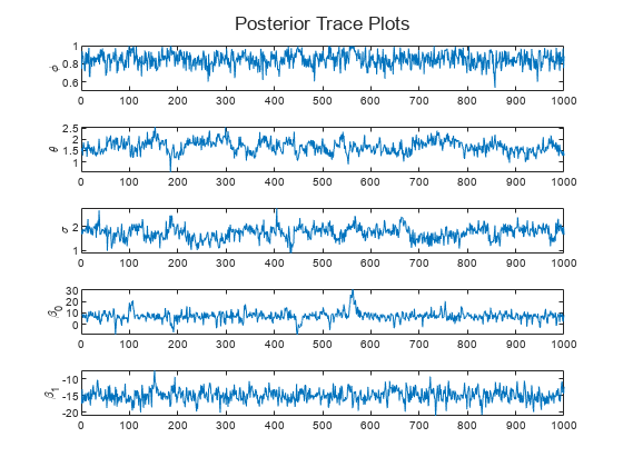
PostParams is a 5-by-1000 matrix of 1000 draws from the posterior distribution. The Metropolis-Hastings sampler accepts 75% of the proposed draws.
paramNames = ["\phi" "\theta" "\sigma" "\beta_0" "\beta_1"];
figure
h = tiledlayout(numParams,1);
for j = 1:numParams
    nexttile
    plot(PostParams(j,:))
    hold on
    ylabel(paramNames(j))
end
title(h,"Posterior Trace Plots")
Input Arguments
Name-Value Arguments
Output Arguments
Algorithms
The Metropolis-Hastings sampler requires a carefully specified proposal distribution. Under the assumption of a Gaussian linear state-space model,
tunetunes the sampler by performing numerical optimization to search for the posterior mode. A reasonable proposal for the multivariate normal or t distribution is the inverse of the negative Hessian matrix, whichtuneevaluates at the resulting posterior mode.When
tunetunes the proposal distribution, the optimizer thattuneuses to search for the posterior mode before computing the Hessian matrix depends on your specifications.
References
Version History
Introduced in R2022a