timescope
Display time-domain signals
Description
The timescope object displays signals in the time
domain.
Scope features:
Data Cursors — Measure signal values using vertical and horizontal cursors.
Signal Statistics — Display the maximum, minimum, peak-to-peak difference, mean, median, and RMS values of a selected signal.
Peak Finder — Find maxima, showing the x-axis values at which they occur.
Bilevel Measurements — Measure transitions, overshoots, undershoots, and cycles.
Triggers — Set triggers to sync repeating signals and pause the display when events occur.
Use Object Functions to show, hide, and determine visibility of the scope window.
You can enable these measurements either programmatically or on the scope UI. For more details, see Measurements.
Creation
Description
scope = timescopetimescope object, scope. This object displays
real- and complex-valued floating and fixed-point signals in the time domain.
scope = timescope(PropertyName=Value)TimeSpan to 100.
Properties
Most properties can be changed from the timescope UI.
Frequently Used
Sampling rate of the input signal, in hertz, specified as a finite numeric scalar or vector of scalars.
The inverse of the sample rate determines the x-axis (time
axis) spacing between points in the displayed signal. When the value of
NumInputPorts is greater than 1 and the sample rate is scalar,
the object uses the same sample rate for all inputs. To specify different sample rates
for each input, use a vector.
You can only set this property when creating the object or after calling
release.
Scope Window Use
On the Scope tab, click Settings, and specify Sample Rate.
Data Types: single | double | int8 | int16 | int32 | int64 | uint8 | uint16 | uint32 | uint64
Source of the time span for frame-based input signals, specified as one of the following:
"property"– The object derives the x-axis limits from theTimeDisplayOffsetandTimeSpanproperties."auto"– The x-axis limits are derived from theTimeDisplayOffsetproperty,SampleRateproperty, and the number of rows in each input signal (FrameSize in the equations below). The limits are calculated as:Minimum time-axis limit =
TimeDisplayOffsetMaximum time-axis limit =
TimeDisplayOffset+ max(1/SampleRate.*FrameSize)
Dependency
When you set the TimeSpan property,
TimeSpanSource is automatically set to
"property".
Scope Window Use
On the Scope tab, click Settings, and
set Time Span to Auto or a positive
scalar.
Data Types: char | string
Time span, in seconds, specified as a positive, numeric scalar value. The time-axis limits are calculated as:
Minimum time-axis limit =
TimeDisplayOffsetMaximum time-axis limit =
TimeDisplayOffset+TimeSpan
Dependencies
To enable this property, set TimeSpanSource to
"property".
Scope Window Use
On the Scope tab, click Settings, and specify Time Span.
Data Types: single | double | int8 | int16 | int32 | int64 | uint8 | uint16 | uint32 | uint64
Specify how the scope displays new data beyond the visible time span as either:
"scroll"— In this mode, the scope scrolls old data to the left to make room for new data on the right of the scope display. This mode is beneficial for debugging and monitoring time-varying signals."wrap"— In this mode, the scope adds data to the left of the plot after overrunning the right of the plot.
Scope Window Use
On the Scope tab, click Settings, and select the overrun behavior in Overrun Action.
Data Types: char | string
Type of plot, specified as one of these:
You can individually control the type of
plot for each line by specifying the PlotType property as a cell
array of character vectors or an array of strings. (since R2025a)
Scope Window Use
On the Scope tab, click Settings, and select Plot Type.
Data Types: char | string
When this property is set to:
"onceatstop"–– The limits are updated once at the end of the simulation (whenreleaseis called)."auto"–– The scope attempts to always keep the data in the display while minimizing the number of updates to the axes limits."manual"–– The scope takes no action unless specified by the user."updates"–– The scope scales the axes once after a set number of visual updates. The number of updates is determined by the value of theAxesScalingNumUpdatesproperty.
Data Types: char | string
Specify the number of updates before scaling as a real, positive scalar integer.
Dependency
To enable this property, set AxesScaling to
"updates".
Data Types: double
Advanced
Specify the layout grid dimensions as a two-element vector:
[numberOfRows,numberOfColumns]. The grid can have a maximum of 10
rows and 10 columns.
If you create a grid of multiple axes, to modify the settings of individual axes,
use the ActiveDisplay.
Example: scope.LayoutDimensions = [2,4]
Scope Window Use
On the Scope tab, click Display Grid (![]() ) and select a specific number of rows and columns in the
grid.
) and select a specific number of rows and columns in the
grid.
Data Types: single | double | int8 | int16 | int32 | int64 | uint8 | uint16 | uint32 | uint64
Specify the units used to describe the x-axis (time axis). You can select one of the following options:
"seconds"—The scope always displays the units on the x-axis as seconds. The scope shows the wordTime(s)on the x-axis."none"— The scope does not display any units on the x-axis. The scope only shows the wordTimeon the x-axis."metric"— The scope displays the units on the x-axis asTime (s)changing the units to day, weeks, months, or years as you plot more data points.
Scope Window Use
On the Scope tab, click Settings, and specify the x-axis units in Time Units.
Data Types: char | string
Specify, in seconds, how far to move the data on the x-axis. The signal value does not change, only the limits displayed on the x-axis change.
If you specify this property as a scalar, then that value is the time display offset for all channels. If you specify this property as a vector, each input signal can have a different time display offset.
Scope Window Use
On the Scope tab, click Settings, and specify Time Offset.
Time-axis labels, specified as:
"all"— Time-axis labels appear in all displays."bottom"— Time-axis labels appear in the bottom display of each column."none"— No labels appear in any display.
Scope Window Use
On the Scope tab, click Settings, and select one of the options in Time Labels.
Data Types: char | string
Specify whether to display the scope in the maximized-axes mode. In this mode, the axes are expanded to fit into the entire display. To conserve space, labels do not appear in each display. Instead, the tick-marks and their values appear on top of the plotted data. You can select one of the following options:
"auto"— The axes appear maximized in all displays only if theTitleandYLabelproperties are empty for every display. If you enter any value in any display for either of these properties, the axes are not maximized."on"— The axes appear maximized in all displays. Any values entered into theTitleandYLabelproperties are hidden."off"— None of the axes appear maximized.
Scope Window Use
On the scope window, click ![]() to maximize axes, hide all labels and inset the
axes values.
to maximize axes, hide all labels and inset the
axes values.
Data Types: char | string
Buffer length, specified as a positive integer. This property sets the number of samples of input data the object keeps for post processing. The post processing actions include zooming after scope stops processing data, panning, and computing measurements.
If the input frame size is greater than the buffer length, the scope stores only
the buffer length number of samples for post processing. To display the entire signal
at once, set the BufferLength property to the length of the input
data.
Scope Window Use
On the Scope tab, click Settings, specify Buffer Length.
Data Types: single | double | int8 | int16 | int32 | int64 | uint8 | uint16 | uint32 | uint64
Measurements
Channel for which to obtain measurements, specified as a positive integer in the range [1 N], where N is the number of input channels.
Scope Window Use
On the Measurements tab, select a Channel.
Data Types: double
Bilevel measurements to measure transitions, aberrations, and cycles of bilevel
signals, specified as a BilevelMeasurementsConfiguration object.
All BilevelMeasurementsConfiguration properties are
tunable.
Scope Window Use
On the Measurements tab, click Bilevel Settings to modify the bilevel measurements.
Cursor measurements to display screen or waveform cursors, specified as a CursorMeasurementsConfiguration object.
All CursorMeasurementsConfiguration properties are
tunable.
Scope Window Use
On the Measurements tab, select Data Cursors to enable the cursors on the display. Click Data Cursors to modify the cursor settings.
Peak finder measurements to compute and display the largest calculated peak
values, specified as a PeakFinderConfiguration object.
All PeakFinderConfiguration
properties are tunable.
Scope Window Use
On the Measurements tab, select Peak Finder to enable the peak finder. Click Peak Finder to modify the peak finder settings.
Signal statistics measurements to compute and display signal statistics, specified
as a SignalStatisticsConfiguration object.
All
SignalStatisticsConfiguration properties are tunable.
Scope Window Use
On the Measurements tab, select Signal Statistics. Click Signal Statistics to choose the statistics to compute.
Trigger measurements, specified as a TriggerConfiguration
object. Define a trigger event to identify the simulation time of specified input
signal characteristics. You can use trigger events to stabilize periodic signals such
as a sine wave or capture non-periodic signals such as a pulse that occurs
intermittently.
All TriggerConfiguration
properties are tunable.
Scope Window Use
On the Measurements tab, select Enable Trigger and click Settings to modify the trigger settings.
Visualization
Specify the name of the scope as a character vector or string scalar. This name
appears as the title of the scope's figure window. To specify a title of a scope plot,
use the Title property.
Data Types: char | string
Scope window position in pixels, specified by the size and location of the scope
window as a four-element vector of the form [left bottom width
height]. You can place the scope window in a specific position on your
screen by modifying the values of this property.
By default, the window appears in the center of your screen with a width of
800 pixels and height of 500 pixels. The exact
values of the position depend on your screen resolution.
Specify the input channel names as a cell array of character vectors or an array
of strings. The channel names appear in the legend, and on the
Measurements tab under Select Channel. If
you do not specify names, the channels are labeled as Channel 1,
Channel 2, etc.
Dependency
To enable this property, set ShowLegend to
true.
Data Types: char
Active display used to set properties, specified by the integer display number.
The number of a display corresponds to the display's row-wise placement index. Setting
this property controls which display is used for the following properties:
YLimits, YLabel,
ShowLegend, ShowGrid,
Title, and PlotAsMagnitudePhase.
Scope Window Use
On the Scope tab, click Settings and specify Active Display.
Specify the display title as a character vector or a string scalar.
Dependency
When you set this property, ActiveDisplay controls the
display that is updated.
Scope Window Use
On the Scope tab, click Settings, and specify Title.
Data Types: char | string
Specify the text for the scope to display to the left of the y-axis.
Dependencies
This property applies only when PlotAsMagnitudePhase is
false. When PlotAsMagnitudePhase is
true, the two y-axis labels are read-only
values "Magnitude" and "Phase", for the
magnitude plot and the phase plot, respectively.
When you set this property, ActiveDisplay controls the
display that is updated.
Scope Window Use
On the Scope tab, click Settings, and specify Y-Label.
Data Types: char | string
Specify the y-axis limits as a two-element numeric vector,
[ymin, ymax].
If
PlotAsMagnitudePhaseisfalse, the default is[-10,10].If
PlotAsMagnitudePhaseistrue, the default is[0,10]. This property specifies the y-axis limits of only the magnitude plot. The y-axis limits of the phase plot are always[-180,180]
Dependency
When you set this property, ActiveDisplay controls the
display that is updated.
Scope Window Use
On the Scope tab, click Settings, and specify Y-Limits.
To show a legend with the input names, set this property to
true.
From the legend, you can control which signals are visible. In the scope legend, click a signal name to hide the signal in the scope. To show the signal, click the signal name again.
Scope Window Use
On the Scope tab, click Legend. Alternatively, click Settings in the Scope tab, and select Show Legend.
Data Types: logical
Set this property to true to show grid lines on the
plot.
Scope Window Use
On the Scope tab, click Settings, and select Show Grid.
Plot signal as magnitude and phased, specified as either:
true– The scope plots the magnitude and phase of the input signal on two separate axes within the same active display.false– The scope plots the real and imaginary parts of the input signal on two separate axes within the same active display.
This property is useful for complex-valued input signals. Turning on this property affects the phase for real-valued input signals. When the amplitude of the input signal is nonnegative, the phase is 0 degrees. When the amplitude of the input signal is negative, the phase is 180 degrees.
Scope Window Use
On the Scope tab, click Settings, and select Magnitude Phase Plot.
Color and Styling
Since R2024b
Background color in scope, specified as an RGB triplet, a hexadecimal color code, a color name, or a short name. For more information on all the acceptable values, see Color.
Tunable: Yes
Scope Window Use
On the Scope tab, click Settings, and select a Background color.
Data Types: double | char
Since R2024b
Color of the axes in the scope, specified as an RGB triplet, a hexadecimal color code, a color name, or a short name. For more information on all the acceptable values, see Color.
Tunable: Yes
Scope Window Use
On the Scope tab, click Settings, and select an Axes color.
Data Types: double | char
Since R2024b
Colors of the labels in the scope, specified as an RGB triplet, a hexadecimal color code, a color name, or a short name. Use this property to set the color of the scope title, x-axis and y-axis labels, and the axes ticks. For more information on all the acceptable values, see Color.
Tunable: Yes
Scope Window Use
On the Scope tab, click Settings, and select a Labels color.
Data Types: double | char
Since R2024b
Scope font size, specified as a positive scalar. Use this property to set the font size for the ticks, labels, title, and measurements of the scope.
Tunable: Yes
Scope Window Use
On the Scope tab, click Settings, and set the Font Size to one of the available values.
Data Types: single | double | int8 | int16 | int32 | int64 | uint8 | uint16 | uint32 | uint64
Since R2024b
Visibility of plot lines in scope, specified as one of these:
"on"or 1 –– The scope displays the plot line. If you are plotting multiple lines, the scope applies this value to all the lines."off"or 0 –– The scope hides the plot line. If you are plotting multiple lines, the scope applies this value to all the lines.vector of logical values –– The scope applies the values to the lines in the plot. The length of the vector must equal the number of lines that you are plotting in the scope.
Tunable: Yes
Scope Window Use
On the Scope tab, click Settings, and select the Visible property.
Data Types: logical
Since R2024b
Scope line style, specified as one of these options:
"-"–– Solid line"--"–– Dashed line":"–– Dotted line"-."–– Dash-dotted line"none"–– No line
If you provide a cell array or an array of these values, then the length of the array must equal the number of lines that you are plotting in the scope.
Tunable: Yes
Scope Window Use
On the Scope tab, click Settings, and set Style.
Since R2024b
Scope line width, specified as a positive scalar or a vector of positive scalar values in points, where 1 point = 1/72 of an inch. If you specify a scalar value and are plotting multiple lines, then the scope applies the same value to all the lines. If you provide a vector of values, the length of the vector must equal the number of lines that you are plotting.
If the line has markers, then the line width also affects the marker edges. The line width cannot be thinner than the width of a pixel. If you set the line width to a value that is less than the width of a pixel on your system, the line displays as one pixel wide.
Tunable: Yes
Scope Window Use
On the Scope tab, click Settings, and set Width.
Data Types: single | double | int8 | int16 | int32 | int64 | uint8 | uint16 | uint32 | uint64
Since R2024b
Scope line color, specified as a matrix of RGB triplets or an array of color names.
Matrix of RGB Triplets
Specify an m-by-3 matrix, where each row is an RGB triplet. An RGB triplet is a three-element vector containing the intensities of the red, green, and blue components of a color. The intensities must be in the range [0,1]. For example, this matrix defines the new colors as blue, dark green, and orange.
scope.LineColor = [1.0 0.0 0.0
                0.0 0.4 0.0
                1.0 0.5 0.0];
Array of Color Names or Hexadecimal Color Codes
Specify any combination of color names, short names, or hexadecimal color codes.
To specify one color, set the line color to a character vector or a string scalar. For example,
scope.LineColor =
                "red"
specifies red as the only color in the color order.To specify multiple colors, set
LineColorto a cell array of character vectors or a string array. For example,scope.LineColor = {"red","green","blue"}specifies red, green, and blue as the colors.
A hexadecimal color code starts with a hash symbol
(#) followed by three or six hexadecimal digits,
which can range from 0 to F. The
values are not case sensitive. Thus, the color codes
"#FF8800", "#ff8800",
"#F80", and "#f80" are
equivalent.
This table lists the color names and short names with the equivalent RGB triplets and hexadecimal color codes.
| Color Name | Short Name | RGB Triplet | Hexadecimal Color Code | Appearance |
|---|---|---|---|---|
"red" | "r" | [1 0 0] | "#FF0000" |
|
"green" | "g" | [0 1 0] | "#00FF00" |
|
"blue" | "b" | [0 0 1] | "#0000FF" |
|
"cyan"
| "c" | [0 1 1] | "#00FFFF" |
|
"magenta" | "m" | [1 0 1] | "#FF00FF" |
|
"yellow" | "y" | [1 1 0] | "#FFFF00" |
|
"black" | "k" | [0 0 0] | "#000000" |
|
"white" | "w" | [1 1 1] | "#FFFFFF" |
|
Scope Window Use
On the Scope tab, click Settings, and set Color.
Tunable: Yes
Data Types: single | double | char | string | cell
Since R2024b
Scope line marker symbol, specified as one of the values listed in this table. By default, the object does not display markers. Specifying a marker symbol adds markers at each data point or vertex.
Tunable: Yes
Scope Window Use
On the Scope tab, click Settings, and set Marker.
Object Functions
To use an object function, specify the object as the first input argument.
hide | Hide scope window |
show | Display scope window |
isVisible | Determine visibility of scope |
generateScript | Generate MATLAB script to create scope with current settings |
printToFigure | Print scope window to MATLAB figure |
step | Run System object algorithm |
release | Release resources and allow changes to System object property values and input characteristics |
reset | Reset internal states of System object |
If you want to restart the simulation from the beginning, call reset to
clear the scope window displays. Do not call reset after calling
release.
Examples
The timescope object requires one of these products:
DSP System Toolbox™
Navigation Toolbox™
Sensor Fusion and Tracking Toolbox™
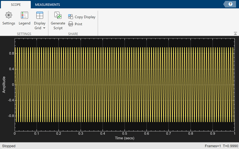
Create a sinusoidal signal with two tones, one at 0.3 kHz and the other at 3 kHz.
t = (0:1000)'/8e3;
xin = sin(2*pi*0.3e3*t)+sin(2*pi*3e3*t);
Create a timescope object and view the sinusoidal signal by calling the time scope object scope.
scope = timescope(SampleRate=8e3,...
    TimeSpanSource="property",...
    TimeSpan=0.1);
scope(xin)
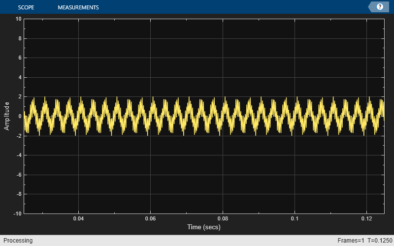
Run release to allow changes to property values and input characteristics. The scope automatically scales the axes.
release(scope);
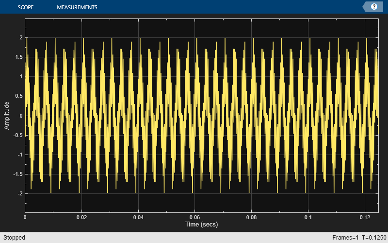
Hide the scope window.
if(isVisible(scope))
    hide(scope)
end
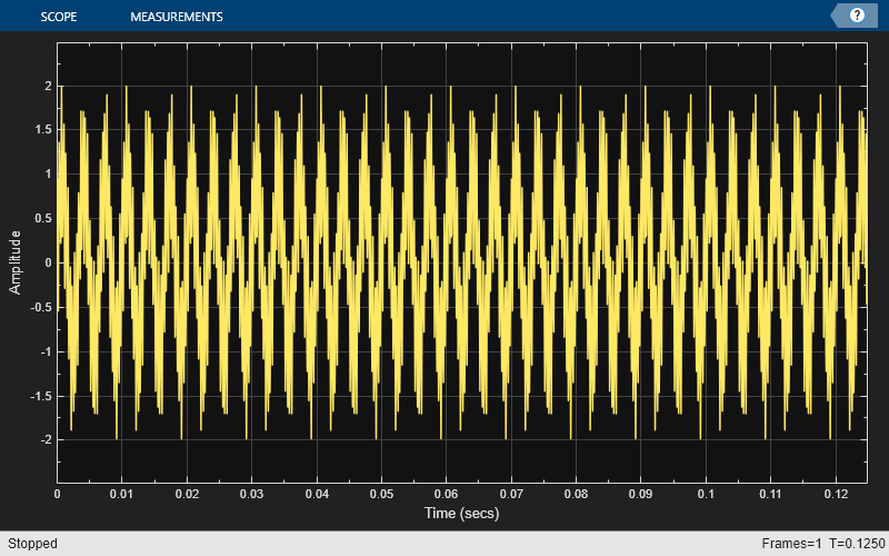
Show the scope window.
if(~isVisible(scope))
    show(scope)
end
Create and Display Clock Input Signal
Load the clock data, x and t. Find the sample time ts.
load clockex
ts = t(2)-t(1);
Create a timescope object and call the object to display the signal.
The timescope object requires one of these products:
DSP System Toolbox™
Navigation Toolbox™
Sensor Fusion and Tracking Toolbox™
scope = timescope(SampleRate=1/ts,TimeSpanSource="auto");
scope(x);
To autoscale the axes and enable changes to property values and input characteristics, call release.
release(scope);
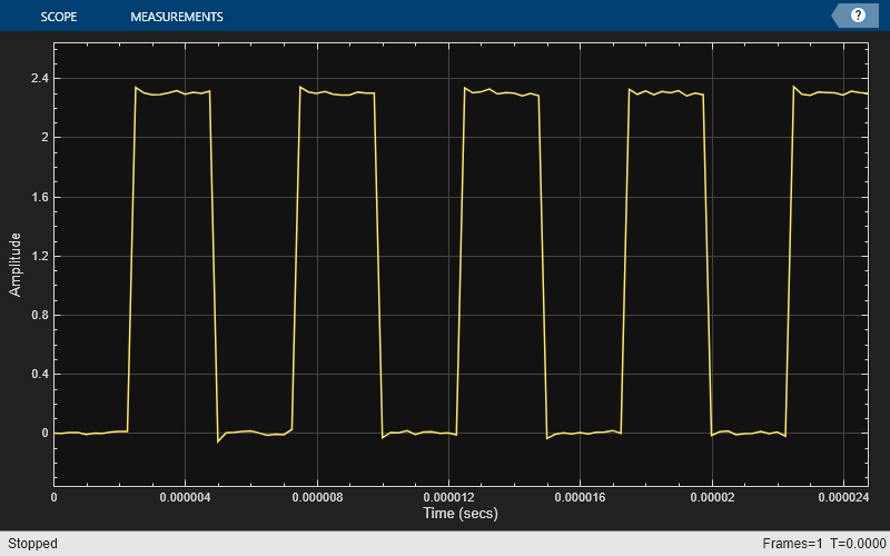
Use Bilevel Measurements Panel to Find Settling Time
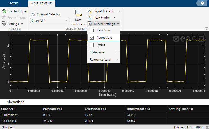
On the Measurements tab, under Bilevel Settings, select Aberrations.
Initially, the Time Scope does not display the Settling Time (s) measurement. This absence occurs because the default value of the Settle Seek (s) parameter is longer than the entire simulation duration.
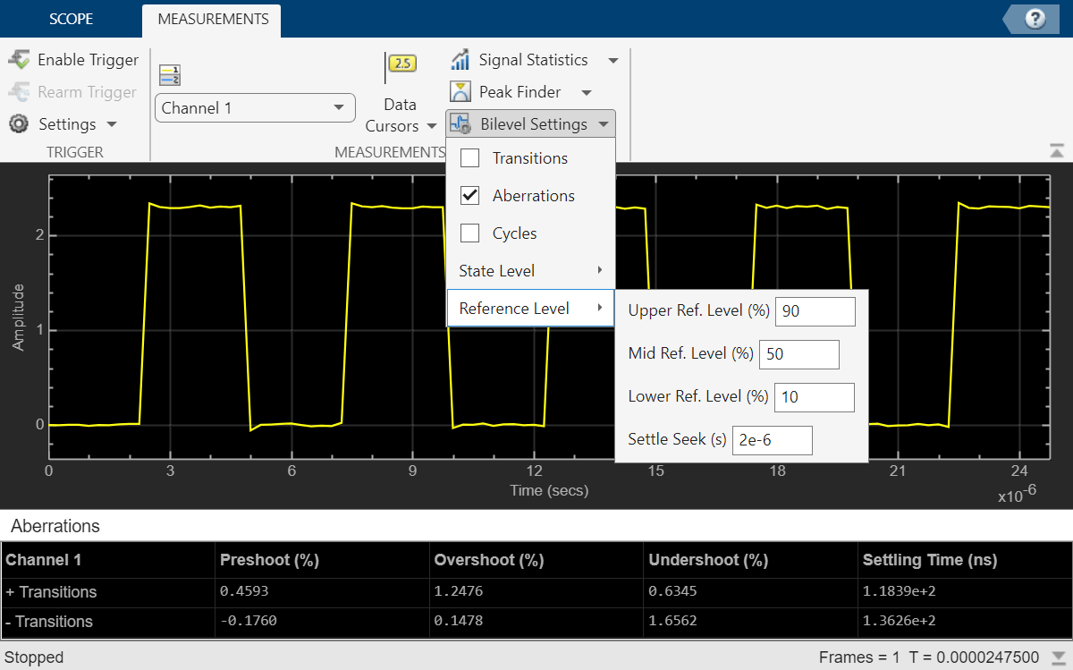
To change the value of the Settle Seek (s) parameter, click Bilevel Settings, and under Reference Level, set the settle seek value to 2e-6 and press Enter.
Time Scope now displays a rising edge Settling Time (ns) value of 118.392 ns.
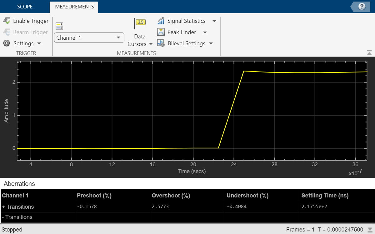
This settling time value is actually the statistical average of the settling times for all five rising edges. To show the settling time for only one rising edge, you can zoom in on that transition.
Hover over the upper right corner of the scope axes and click the zoom button.
Click and drag to zoom in on one of the transitions. Set Settle Seek (s) to 2e-7 and press Enter.
The Time Scope updates the rising edge Settling Time value to reflect the new time window.
Create a sine wave and view it in the Time Scope. Programmatically compute the bilevel measurements related to signal transitions, aberrations, and cycles.
The timescope object requires one of these products:
DSP System Toolbox™
Navigation Toolbox™
Sensor Fusion and Tracking Toolbox™
Initialization
Create the input sine wave using the sin function. Create a timescope MATLAB® object to display the signal. Set the TimeSpan property to 1 second.
f = 100;
fs = 1000;
swv = sin(2.*pi.*f.*(0:1/fs:1-1/fs)).';
scope = timescope(SampleRate=fs,...
    TimeSpanSource="property",...
    TimeSpan=1);
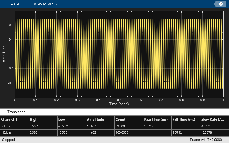
Transition Measurements
Enable the scope to show transition measurements programmatically by setting the ShowTransitions property to true. Display the sine wave in the scope.
Transition measurements such as rise time, fall time, and slew rate appear in the Transitions pane at the bottom of the scope.
scope.BilevelMeasurements.ShowTransitions = true;
scope(swv);
release(scope);
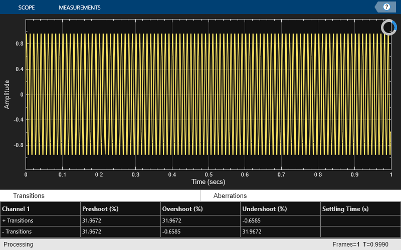
Aberration Measurements
Enable the scope to show aberration measurements programmatically by setting the ShowAberrations property to true. Display the sine wave in the scope.
Aberration measurements such as preshoot, overshoot, undershoot, and settling time appear in the Aberrations pane at the bottom of the scope.
scope.BilevelMeasurements.ShowAberrations = true;
scope(swv);
release(scope);
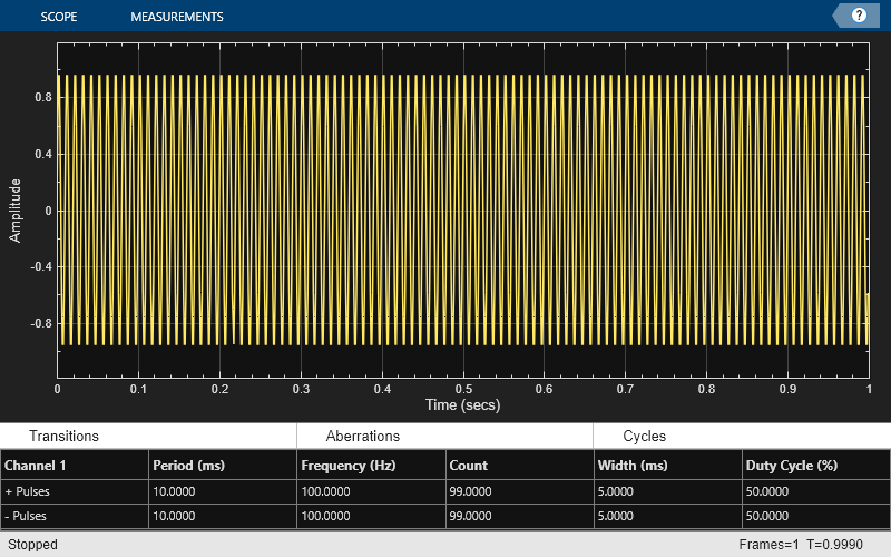
Cycle Measurements
Enable the scope to show cycles measurements programmatically by setting the ShowCycles property to true. Display the sine wave in the scope.
Cycle measurements such as period, frequency, pulse width, and duty cycle appear in the Cycles pane at the bottom of the scope.
scope.BilevelMeasurements.ShowCycles = true;
scope(swv);
release(scope);
Create a sine wave and view it in the Time Scope. Enable the scope programmatically to compute the signal statistics.
The timescope object requires one of these products:
DSP System Toolbox™
Navigation Toolbox™
Sensor Fusion and Tracking Toolbox™
The timescope object supports these signal statistics:
Maximum
Minimum
Mean
Median
RMS
Peak to peak
Variance
Standard deviation
Mean square
Initialization
Create the input sine wave using the sin function. Create a timescope MATLAB® object to display the signal. Set the TimeSpan property to 1 second.
f = 100;
fs = 1000;
swv = sin(2.*pi.*f.*(0:1/fs:1-1/fs)).';
scope = timescope(SampleRate=fs,...
    TimeSpanSource="property",...
    TimeSpan=1);
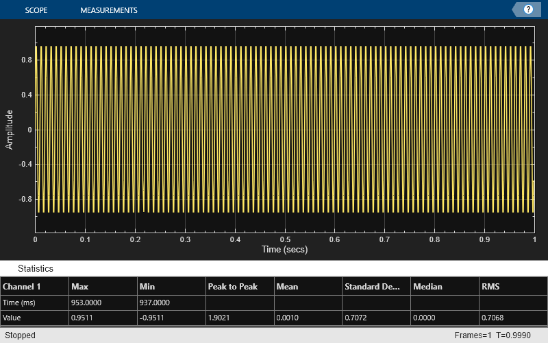
Signal Statistics
Enable the scope to show signal statistics programmatically by setting the SignalStatistics > Enabled property to true.
scope.SignalStatistics.Enabled = true;
By default, the scope enables the following measurements.
scope.SignalStatistics
ans =
  SignalStatisticsConfiguration with properties:

                  ShowMax: 1
                  ShowMin: 1
           ShowPeakToPeak: 1
                 ShowMean: 1
             ShowVariance: 0
    ShowStandardDeviation: 1
               ShowMedian: 1
                  ShowRMS: 1
           ShowMeanSquare: 0
                  Enabled: 1
Display the sine wave in the scope. A Statistics pane appears at the bottom of the scope window displaying the statistics for the portion of the signal that you can see in the scope.
If you use the zoom options on the scope, the statistics automatically adjust to the time range in the display.
scope(swv);
release(scope);
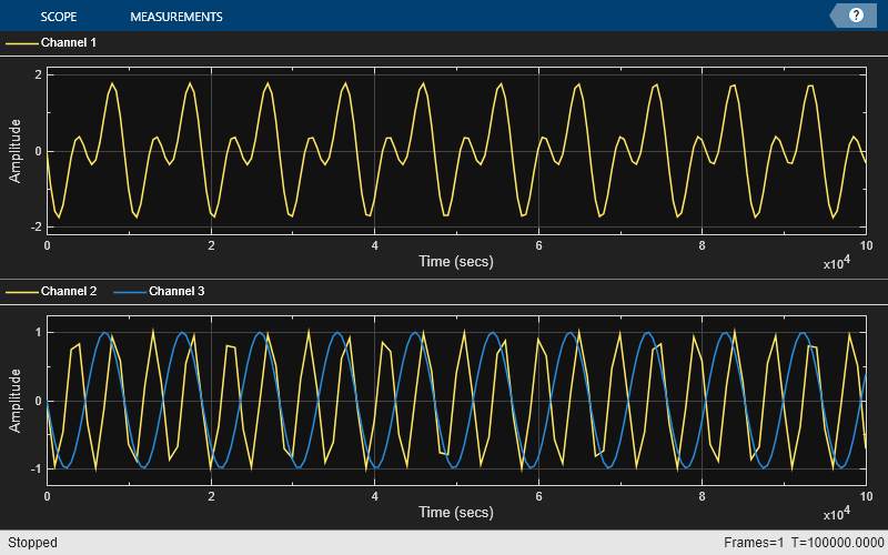
This example shows how to visualize multiple inputs with different sample rates and plot the signals on multiple axes.
Generate three different sine waves and plot them in the Time Scope.
The timescope object requires one of these products:
DSP System Toolbox™
Navigation Toolbox™
Sensor Fusion and Tracking Toolbox™
freq = 1/500;
t    = (0:100)'/freq;
t2   = (0:0.5:100)'/freq;
xin1 = sin(1/2*t);
xin2 = sin(1/4*t2);
xin  = sin(1/2*t2)+sin(1/4*t2);

scope = timescope(SampleRate=[freq freq/2 freq],...
    TimeSpanSource="property", ...
    TimeSpan=0.1,...
    LayoutDimensions=[2,1]);
scope(xin,xin1,xin2)

release(scope)
This example show how to add titles, set y-axis limits, and modify properties when you have multiple axes on your timescope object.
The timescope object requires one of these products:
DSP System Toolbox™
Navigation Toolbox™
Sensor Fusion and Tracking Toolbox™
Use the timescope object to visualize three sine waves with two different sample rates.
freq = 1;
t    = (0:100)'/freq;
t2   = (0:0.5:100)'/freq;
xin1 = sin(1/2*t);
xin2 = sin(1/4*t2);
xin  = sin(1/2*t2)+sin(1/4*t2);

scope = timescope(SampleRate=[freq freq/2 freq],...
     TimeSpanSource="property",...
     TimeSpan=100);
scope(xin, xin1, xin2)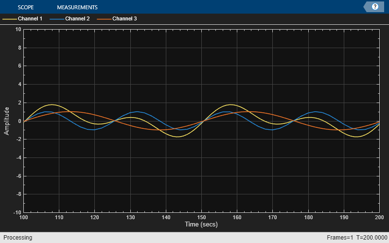
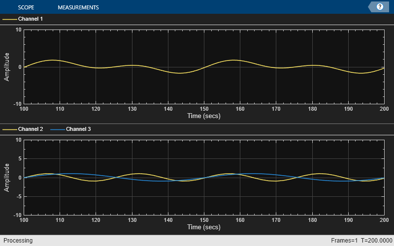
Change the layout to add a second axis. The second and third inputs automatically move to the new second axis.
scope.LayoutDimensions = [2,1];
Modify the properties of the first axis.
scope.ActiveDisplay = 1;
scope.ShowGrid = false;
scope.Title = "Sine Wave 1";
scope.YLimits = [-2,2];
Repeat this process to modify the second axis.
scope.ActiveDisplay = 2;
scope.Title = "Sine Waves 2 & 3";
scope.YLimits = [-1,1];
release(scope)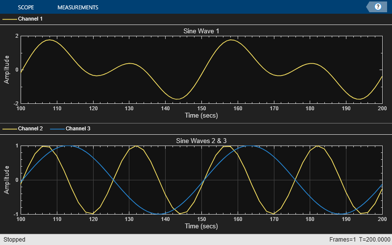
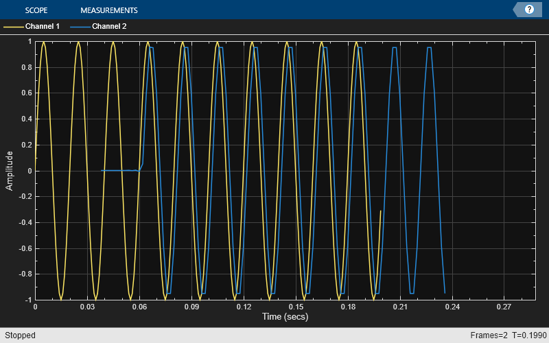
Create a dsp.SineWave object. Create a dsp.FIRDecimator object to decimate the sine wave by 2. Create a timescope object with two input ports.
Fs = 1000;  % Sample rate
sine = dsp.SineWave(Frequency=50,...
   SampleRate=Fs,...
   SamplesPerFrame=100);
decimate = dsp.FIRDecimator; % To decimate sine by 2
scope = timescope(SampleRate=[Fs Fs/2],...
   TimeDisplayOffset=[0 38/Fs],...
   TimeSpanSource="Property",...
   TimeSpan=0.25,...
   YLimits=[-1 1],...
   ShowLegend=true);
Call the dsp.SineWave object to create a sine wave signal. Use the dsp.FIRDecimator object to create a second signal that equals the original signal and decimate it by a factor of 2. Display the signals by calling the timescope object.
for ii = 1:2
     xsine = sine();
     xdec = decimate(xsine);
     scope(xsine,xdec)
end
release(scope)
Close the Time Scope window and clear the variables.
clear scope Fs sine decimate ii xsine xdec
Create a vector representing a complex-valued sinusoidal signal and a timescope object. Call the scope to display the signal.
The timescope object requires one of these products:
DSP System Toolbox™
Navigation Toolbox™
Sensor Fusion and Tracking Toolbox™
fs = 1000;
t = (0:1/fs:10)';
CxSine = cos(2*pi*0.2*t) + 1i*sin(2*pi*0.2*t);
CxSineSum = cumsum(CxSine);
scope = timescope(SampleRate=fs,...
TimeSpanSource="auto",ShowLegend=1);
scope(CxSineSum);
release(scope)
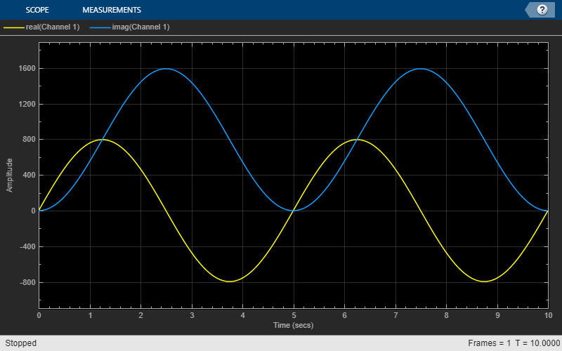
By default, when the input is a complex-valued signal, the Time Scope plots the real and imaginary portions on the same axes. These portions appear as different-colored lines on the same axes within the same active display.
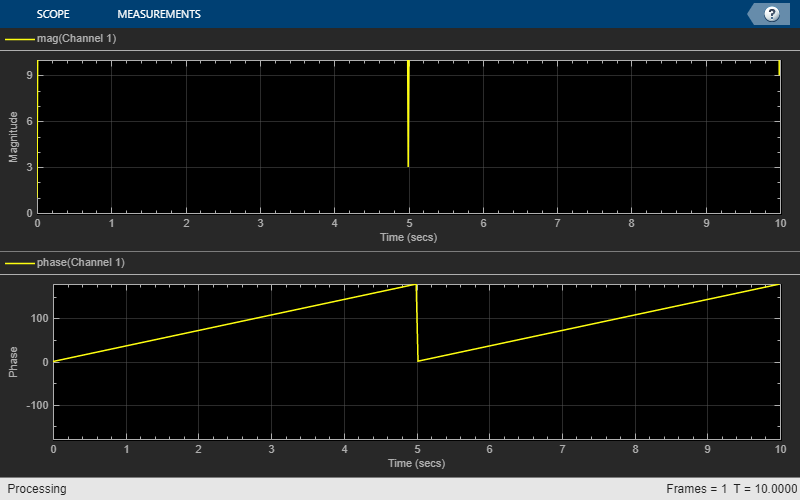
Change the PlotAsMagnitudePhase property to true and call release.
The Time Scope now plots the magnitude and phase of the input signal on two separate axes within the same active display. The top axes display magnitude and the bottom axes display the phase in degrees.
scope.PlotAsMagnitudePhase = true;
scope(CxSineSum);
release(scope)
This example shows how the timescope object visualizes inputs that change dimensions halfway through.
The timescope object requires one of these products:
DSP System Toolbox™
Navigation Toolbox™
Sensor Fusion and Tracking Toolbox™
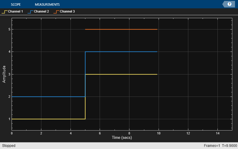
Create a vector that represents a two-channel constant signal. Create another vector that represents a three-channel constant signal. Create a timescope object and call the scope with two inputs to display the signal.
fs = 10;
sigdim2 = [ones(5*fs,1) 1+ones(5*fs,1)];                   % 2-dim 0-5 s
sigdim3 = [2+ones(5*fs,1) 3+ones(5*fs,1) 4+ones(5*fs,1)];  % 3-dim 5-10 s
scope = timescope(SampleRate=fs,TimeSpanSource="property");
scope.PlotType = "stairs";
scope.TimeSpanOverrunAction = "scroll";
scope.TimeDisplayOffset = [0 5];
scope([sigdim2; sigdim3(:,1:2)], sigdim3(:,3));
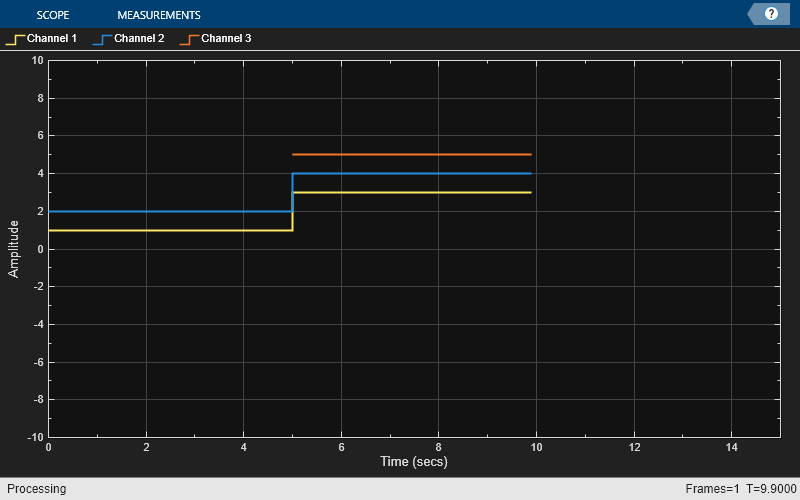
The size of the input signal to the Time Scope changes as the simulation progresses. When the simulation time is less than 5 seconds, the Time Scope plots only the two-channel signal sigdim2. After 5 seconds, the Time Scope also plots the three-channel signal sigdim3.
Run the release method to enable changes to property values and input characteristics. The scope automatically scales the axes.
release(scope)
Use Peak Finder pane in the Time Scope to measure heart rate.
The sgolayfilt function requires the Signal Processing Toolbox™.
The timescope object requires one of these products:
DSP System Toolbox™
Navigation Toolbox™
Sensor Fusion and Tracking Toolbox™
Create and Display ECG Signal
Use the custom ecg function to generate an electrocardiogram (ECG) signal.
type ecg.mfunction x = ecg(L)
a0 = [0, 1, 40, 1, 0, -34, 118, -99, 0, 2, 21, 2, 0, 0, 0];
d0 = [0, 27, 59, 91, 131, 141, 163, 185, 195, 275, 307, 339, 357, 390, 440];
a = a0 / max(a0);
d = round(d0 * L / d0(15));
d(15) = L;
for i = 1:14
m = d(i) : d(i+1) - 1;
slope = (a(i+1) - a(i)) / (d(i+1) - d(i));
x(m+1) = a(i) + slope * (m - d(i));
end
x1 = 3.5*ecg(2700).';
y1 = sgolayfilt(kron(ones(1,13),x1),0,21);
n = (1:30000)';
del = round(2700*rand(1));
mhb = y1(n + del);
ts = 0.00025;
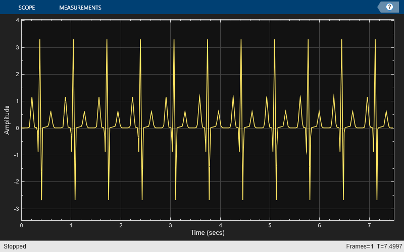
Create a timescope object and call the object to display the signal. To autoscale the axes and enable changes to property values and input characteristics, call release.
scope = timescope(SampleRate=1/ts);
scope(mhb);
release(scope)
Find Heart Rate
Use the Peak Finder measurements to measure the time between heartbeats.
In the Measurements tab, select Peak Finder to enable the peak finder measurements.
Click the Peak Finder arrow and set the Num Peaks property to 10 and hit enter.
In the Peaks pane at the bottom of the window, the Time Scope displays a list of ten peak amplitude values and the times at which they occur.
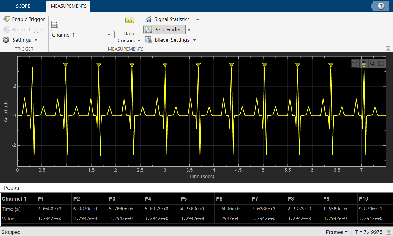
The list of peak values shows a constant time difference of 0.675 seconds between each heartbeat. Based on this equation, the heart rate of this ECG signal is about 89 beats per minute.
Close the Time Scope window and remove the variables you created from the workspace.
clear scope x1 y1 n del mhb ts
Since R2024b
Create a timescope object. The input signals are a set of four sinusoidal signals.
The timescope object requires one of these products:
DSP System Toolbox™
Navigation Toolbox™
Sensor Fusion and Tracking Toolbox™
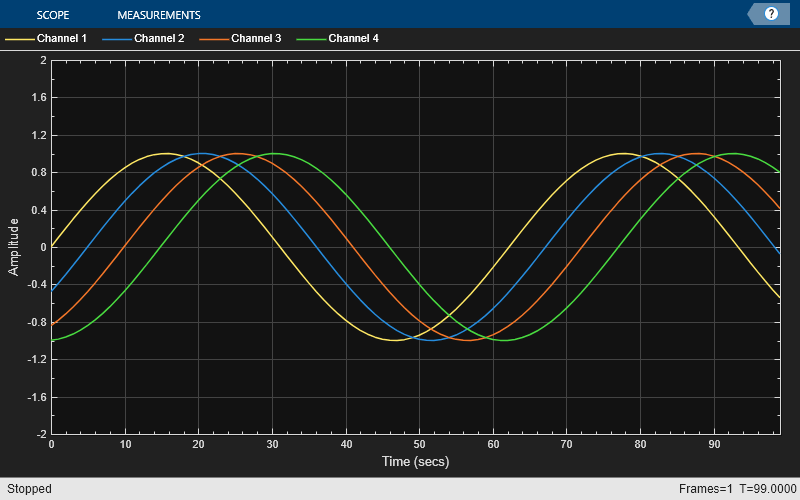
ts = timescope(YLimits=[-2 2]);
x = linspace(0,10).';
y1 = sin(x);
y2 = sin(x-0.5);
y3 = sin(x-1);
y4 = sin(x-1.5);
Visualize the signals in the time scope. This plot shows the default color and style settings of the timescope object.
ts(y1,y2,y3,y4);
release(ts);
Change the background color and the axes color of the plot to "white". Set the font color to "black". Also, change the line colors to ["red" "green" "black" "magenta"].
ts.BackgroundColor = "white";
ts.AxesColor = "white";
ts.FontColor = "black";
ts.LineColor = ["red" "green" "black" "magenta"];
show(ts)
release(ts)

To change the color order, set LineColor to a different color order. This setting changes the color order palette.
ts.LineColor = colororder("glow");
show(ts)
release(ts)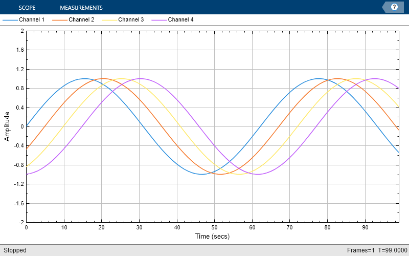
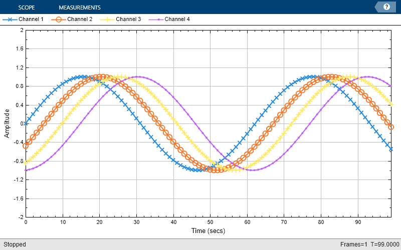
You can further specify a marker for each line and change the corresponding line width.
ts.LineMarker = ["x","o","+","."];
ts.LineWidth = 2;
show(ts)
release(ts)
To control the visibility of the plot lines, use the LineVisible property. When you select "off", the plot line becomes invisible.
ts.LineVisible = ["off" "on" "on" "off"];
show(ts)
release(ts)

Since R2023b
Use the printToFigure function to print the timescope object display window to a new MATLAB® figure.
The timescope object requires one of these products:
DSP System Toolbox™
Navigation Toolbox™
Sensor Fusion and Tracking Toolbox™
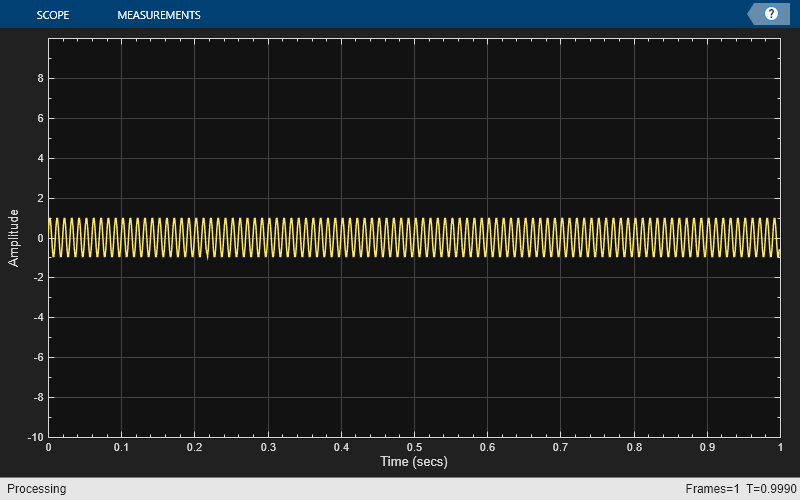
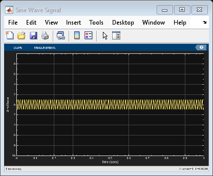
View a sine wave on the time scope. This plot shows the default color and style settings of the timescope object.
f = 100;
fs = 1000;
swv = sin(2.*pi.*f.*(0:1/fs:1-1/fs)).';
scope = timescope(SampleRate=fs,...
    TimeSpanSource="property", ...
    TimeSpan=1);
scope(swv);
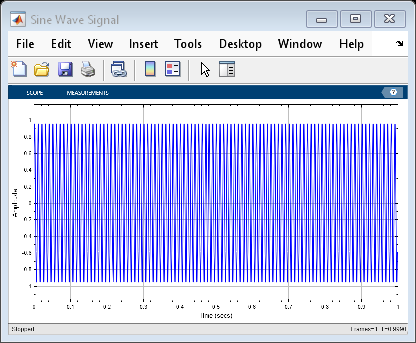
Change the background color and the axes color of the plot to "white". Set the font color to "black" and the line color to "blue".
scope.BackgroundColor = "white";
scope.AxesColor = "white";
scope.FontColor = "black";
scope.LineColor = "blue";
show(scope)
release(scope)
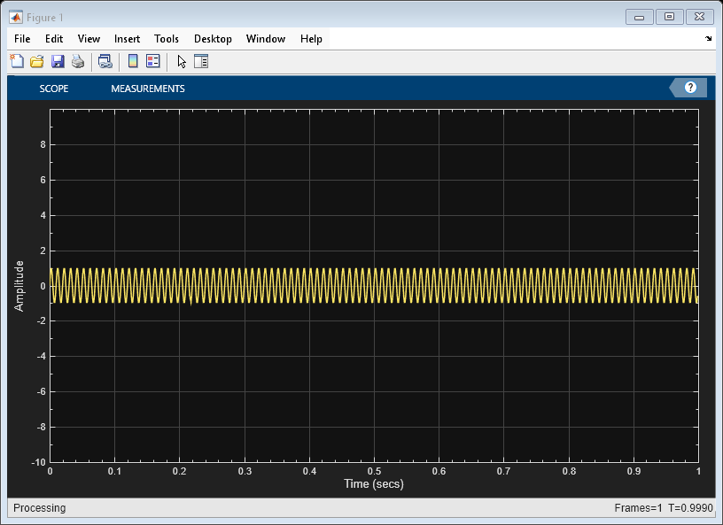
Print the display of the sine wave to a new MATLAB figure. The function returns a handle to the figure.
scopeFig = printToFigure(scope);
The handle to the figure scopeFig lets you modify the appearance and the behavior of the figure window.
Specify a figure name and change the size of the figure to 400-by-250 pixels.
scopeFig.Name="Sine Wave Signal";
scopeFig.NumberTitle="off";
scopeFig.Position=[1 1 400 250];
When printing to figure, you can make the figure invisible by setting the Visible argument to false.
scopeFig = printToFigure(scope,Visible=false);
Limitations
Does not support C/C++ code generation using MATLAB® Coder™. To generate a standalone application, use the MATLAB Compiler™.
Supports MEX code generation by treating the calls to the object as extrinsic.
Tips
To close the scope window and clear its associated data, use the MATLAB
clearfunction.To hide or show the scope window, use the
hideandshowfunctions.Use the MATLAB
mccfunction to compile code containing a scope. You cannot open scope configuration dialog boxes if you have more than one compiled component in your application.