msesim
Estimated mean squared error for adaptive filters
Syntax
Description
Examples
The mean squared error (MSE) measures the average of the squares of the errors between the desired signal and the primary signal input to the adaptive filter. Reducing this error converges the primary input to the desired signal. Determine the predicted value of MSE and the simulated value of MSE at each time instant using the msepred and msesim functions. Compare these MSE values with each other and with respect to the minimum MSE and steady-state MSE values. In addition, compute the sum of the squares of the coefficient errors given by the trace of the coefficient covariance matrix.
Initialization
Create a dsp.FIRFilter System object™ that represents the unknown system. Pass the signal, x, to the FIR filter. The output of the unknown system is the desired signal, d, which is the sum of the output of the unknown system (FIR filter) and an additive noise signal, n.
num = fir1(31,0.5);
fir = dsp.FIRFilter('Numerator',num);
iir = dsp.IIRFilter('Numerator',sqrt(0.75),...
        'Denominator',[1 -0.5]);
x = iir(sign(randn(2000,25)));
n = 0.1*randn(size(x));
d = fir(x) + n;
LMS Filter
Create a dsp.LMSFilter System object to create a filter that adapts to output the desired signal. Set the length of the adaptive filter to 32 taps, step size to 0.008, and the decimation factor for analysis and simulation to 5. The variable simmse represents the simulated MSE between the output of the unknown system, d, and the output of the adaptive filter. The variable mse gives the corresponding predicted value.
l = 32;
mu = 0.008;
m  = 5;

lms = dsp.LMSFilter('Length',l,'StepSize',mu);
[mmse,emse,meanW,mse,traceK] = msepred(lms,x,d,m);
[simmse,meanWsim,Wsim,traceKsim] = msesim(lms,x,d,m);
Plot the MSE Results
Compare the values of simulated MSE, predicted MSE, minimum MSE, and the final MSE. The final MSE value is given by the sum of minimum MSE and excess MSE.
nn = m:m:size(x,1);
semilogy(nn,simmse,[0 size(x,1)],[(emse+mmse)...
    (emse+mmse)],nn,mse,[0 size(x,1)],[mmse mmse])
title('Mean Squared Error Performance')
axis([0 size(x,1) 0.001 10])
legend('MSE (Sim.)','Final MSE','MSE','Min. MSE')
xlabel('Time Index')
ylabel('Squared Error Value')
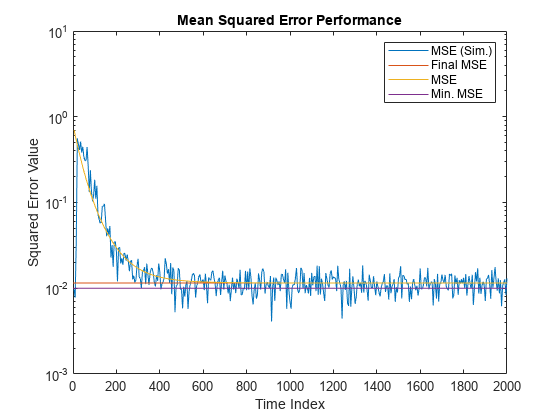
The predicted MSE follows the same trajectory as the simulated MSE. Both these trajectories converge with the steady-state (final) MSE.
Plot the Coefficient Trajectories
meanWsim is the mean value of the simulated coefficients given by msesim. meanW is the mean value of the predicted coefficients given by msepred.
Compare the simulated and predicted mean values of LMS filter coefficients 12,13,14, and 15.
plot(nn,meanWsim(:,12),'b',nn,meanW(:,12),'r',nn,...
meanWsim(:,13:15),'b',nn,meanW(:,13:15),'r')
PlotTitle ={'Average Coefficient Trajectories for';...
            'W(12), W(13), W(14), and W(15)'}
PlotTitle = 2×1 cell
    {'Average Coefficient Trajectories for'}
    {'W(12), W(13), W(14), and W(15)'      }
title(PlotTitle)
legend('Simulation','Theory')
xlabel('Time Index')
ylabel('Coefficient Value')
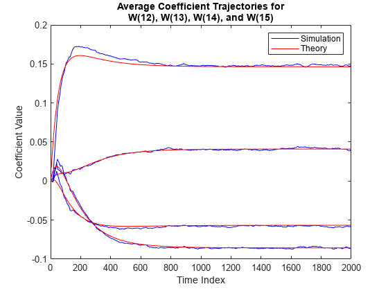
In steady state, both the trajectories converge.
Sum of Squared Coefficient Errors
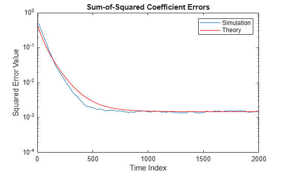
Compare the sum of the squared coefficient errors given by msepred and msesim. These values are given by the trace of the coefficient covariance matrix.
semilogy(nn,traceKsim,nn,traceK,'r')
title('Sum-of-Squared Coefficient Errors')
axis([0 size(x,1) 0.0001 1])
legend('Simulation','Theory')
xlabel('Time Index')
ylabel('Squared Error Value')
Identify an unknown system by performing active noise control using a filtered-x LMS algorithm. The objective of the adaptive filter is to minimize the error signal between the output of the adaptive filter and the output of the unknown system (or the system to be identified). Once the error signal is minimal, the unknown system converges to the adaptive filter.
Initialization
Create a dsp.FIRFilter System object that represents the system to be identified. Pass the signal, x, to the FIR filter. The output of the unknown system is the desired signal, d, which is the sum of the output of the unknown system (FIR filter) and an additive noise signal, n.
num = fir1(31,0.5);
fir = dsp.FIRFilter(Numerator=num);
iir = dsp.IIRFilter(Numerator=sqrt(0.75),...
        Denominator=[1 -0.5]);
x = iir(sign(randn(2000,25)));
n = 0.1*randn(size(x));
d = fir(x) + n;
Adaptive Filter
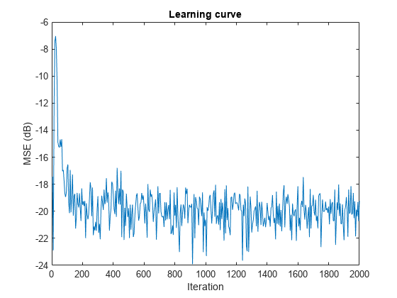
Create a dsp.FilteredXLMSFilter System object to create an adaptive filter that uses the filtered-x LMS algorithm. Set the length of the adaptive filter to 32 taps, step size to 0.008, and the decimation factor for analysis and simulation to 5. The variable simmse represents the error between the output of the unknown system, d, and the output of the adaptive filter.
l = 32;
mu = 0.008;
m  = 5;
fxlms = dsp.FilteredXLMSFilter(l,StepSize=mu);
[simmse,meanWsim,Wsim,traceKsim] = msesim(fxlms,x,d,m);
plot(m*(1:length(simmse)),10*log10(simmse))
xlabel("Iteration")
ylabel("MSE (dB)")
% Plot the learning curve for filtered-x LMS filter
% used in system identification
title("Learning curve")
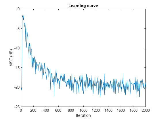
With each iteration of adaptation, the value of simmse decreases to a minimal value, indicating that the unknown system has converged to the adaptive filter.
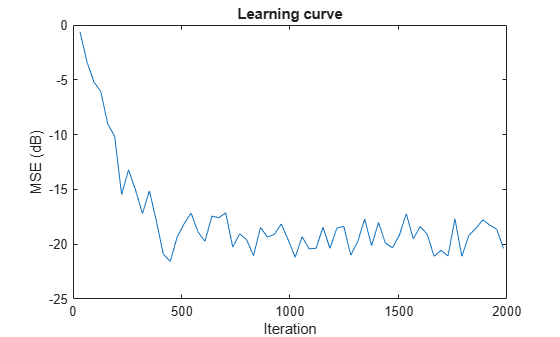
ha = fir1(31,0.5);
% FIR system to be identified
fir = dsp.FIRFilter(Numerator=ha);
iir = dsp.IIRFilter(Numerator=sqrt(0.75),...
        Denominator=[1 -0.5]);
x = iir(sign(randn(2000,25)));
% Observation noise signal
n = 0.1*randn(size(x));
 % Desired signal
d = fir(x)+n;
% Filter length
l = 32;
% Decimation factor for analysis
% and simulation results
m  = 5;
ha = dsp.AdaptiveLatticeFilter(l);
[simmse,meanWsim,Wsim,traceKsim] = msesim(ha,x,d,m);
plot(m*(1:length(simmse)),10*log10(simmse));
xlabel("Iteration");
ylabel("MSE (dB)");
% Plot the learning curve used for
% adaptive lattice filter used in system identification
title("Learning Curve")
fir = fir1(31,0.5);
% FIR system to be identified
firFilter = dsp.FIRFilter(Numerator=fir);
iirFilter = dsp.IIRFilter(Numerator=sqrt(0.75),...
        Denominator=[1 -0.5]);
x = iirFilter(sign(randn(2000,25)));
% Observation noise signal
n = 0.1*randn(size(x));
% Desired signal
d = firFilter(x)+n;
% Filter length
l = 32;
% Block LMS Step size
mu = 0.008;
% Decimation factor for analysis
% and simulation results
m  = 32;
fir = dsp.BlockLMSFilter(l,StepSize=mu);
[simmse,meanWsim,Wsim,traceKsim] = msesim(fir,x,d,m);
plot(m*(1:length(simmse)),10*log10(simmse));
xlabel("Iteration"); ylabel("MSE (dB)");
% Plot the learning curve for
% block LMS filter used in system identification
title("Learning curve")
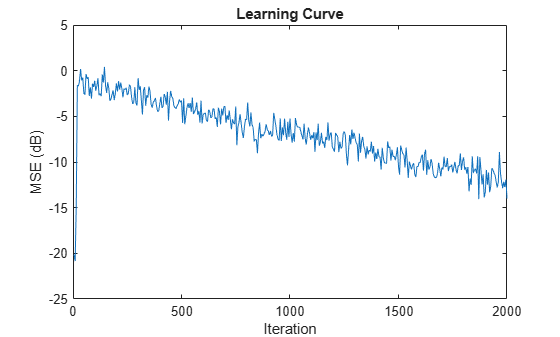
ha = fir1(31,0.5);
% FIR system to be identified
fir = dsp.FIRFilter(Numerator=ha);
iir = dsp.IIRFilter(Numerator=sqrt(0.75),...
        Denominator=[1 -0.5]);
x = iir(sign(randn(2000,25)));
% Observation noise signal
n = 0.1*randn(size(x));
% Desired signal
d = fir(x)+n;
% Filter length
l = 32;
% Affine Projection filter Step size.
mu = 0.008;
% Decimation factor for analysis
% and simulation results
m  = 5;

apf = dsp.AffineProjectionFilter(l,"StepSize",mu);
[simmse,meanWsim,Wsim,traceKsim] = msesim(apf,x,d,m);
plot(m*(1:length(simmse)),10*log10(simmse));
xlabel("Iteration"); ylabel("MSE (dB)");
% Plot the learning curve for affine projection filter
% used in system identification
title("Learning Curve")
Input Arguments
Output Arguments
References
[1] Hayes, M.H. Statistical Digital Signal Processing and Modeling. New York: John Wiley & Sons, 1996.
Version History
Introduced in R2012a